Bernoulli numbers appear as coefficients in formulas for sums of powers of natural numbers.
For example:
$$
1 + 2 + \cdots + n = \frac{1}{2}B_0\,n^2 + B_1\,n
$$
The zeta function is also related to Bernoulli numbers through the formula
$$
\zeta(1-s) = -\frac{B_s}{s}.
$$
This page explains how the zeta function assigns the value -1/12 to the divergent series of natural numbers.
• Why the natural-number series of the zeta function does not simply diverge (2014/2/8)
In 1644, the Italian mathematician Pietro Mengoli asked for the value of the series
$$ \frac{1}{1^2} + \frac{1}{2^2} + \frac{1}{3^2} + \cdots. $$The Swiss mathematician Jacob Bernoulli tried to solve the problem but could not find the answer. The question later became known as the Basel problem, after Bernoulli's hometown of Basel.
In 1735, at the age of 28, Leonhard Euler solved the problem and showed that
$$ \frac{1}{1^2} + \frac{1}{2^2} + \frac{1}{3^2} + \cdots = \frac{\pi^2}{6}. $$This was a remarkable result, because it connected a simple infinite series with the geometry of circles. Later, in 1749, Euler discovered an even more surprising identity:
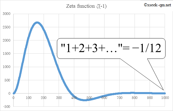
$$ 1 + 2 + 3 + \cdots = -\frac{1}{12}. $$At first sight this looks impossible: in the ordinary sense, the series diverges. How, then, can a finite value be assigned to it? In 1913, the Indian mathematician Srinivasa Ramanujan developed a summation method that helps explain this result.
First, consider the series
Using a shift-and-add argument, we obtain
Next, define the alternating series
Applying a similar shift-and-add argument gives
Finally, consider the series of natural numbers:
Multiplying by four and subtracting gives
Of course, the ordinary series 1 + 2 + 3 + ··· diverges, so this manipulation is not rigorous in the usual sense. One way to make the idea precise is to introduce a damping factor, as illustrated below.
Define the damped sum
$$ H_n(x) = \sum_{k=1}^n k\,e^{-kx}\cos(kx). $$For finite n, as x → 0⁺, Hn(x) approaches 1 + 2 + … + n. However, if we first take the infinite sum and then let x approach 0⁺, the value becomes −1/12:
$$ \lim_{x\to0^+}\sum_{k=1}^\infty k\,e^{-kx}\cos(kx) = -\frac{1}{12}. $$You can check this limit numerically on Wolfram|Alpha:
For more details on this method, see:
This kind of regularization also appears in calculations of the Casimir effect, where it allows one to handle quantities that would otherwise be expressed as divergent sums.
In 2015, NS proposed the following general regularization formula:
$$ \zeta(1-2t) = \lim_{x\to0^+}\sum_{k=1}^\infty \frac{1}{k^{1-2t}}\,e^{-k^t x}\cos(k^t x). $$For example, setting t=2 gives ζ(−3)=1/120.
In 1859, Bernhard Riemann defined the zeta function for s by
$$ \zeta(s) = \sum_{n=1}^\infty \frac{1}{n^s}, $$and extended it analytically to the complex plane using
$$ \zeta(s) = \Gamma(1-s)\oint_{C}\frac{dz}{2\pi i\,z}\,z^s\frac{e^z}{1-e^z}. $$The integral gives the global zeta function, while the original series is often denoted Z(s):
$$ Z(s) = \sum_{n=1}^\infty \frac{1}{n^s}. $$Riemann's reflection formula connects these two expressions:
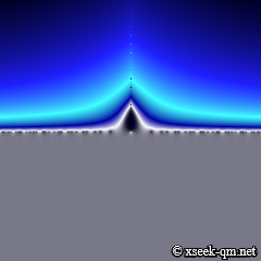
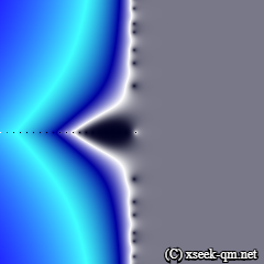
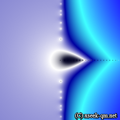
$$ \zeta(1-s) = \frac{2}{(2\pi)^s}\,\Gamma(s)\,\cos\!\bigl(\tfrac{\pi s}{2}\bigr)\,\zeta(s). $$From this formula, one can derive ζ(−1)=−1/12. The graph below shows the global zeta function.
If the image is rotated and enlarged, it resembles a mountainous landscape under a blue sky. Riemann conjectured that every nontrivial zero has real part 1/2. This is the Riemann Hypothesis. The first few nontrivial zeros are:
Bernoulli numbers first appeared in formulas for sums of powers of natural numbers. For powers 0 through 6, the formulas are:
| $$1^0 + 2^0 + 3^0 + \cdots + n^0 = \frac{1}{1}n^1$$ |
| $$1^1 + 2^1 + 3^1 + \cdots + n^1 = \frac{1}{2}n^2 + \frac{1}{2}n^1$$ |
| $$1^2 + 2^2 + 3^2 + \cdots + n^2 = \frac{1}{3}n^3 + \frac{1}{2}n^2 + \frac{1}{6}n^1$$ |
| $$1^3 + 2^3 + 3^3 + \cdots + n^3 = \frac{1}{4}n^4 + \frac{1}{2}n^3 + \frac{1}{4}n^2$$ |
| $$1^4 + 2^4 + 3^4 + \cdots + n^4 = \frac{1}{5}n^5 + \frac{1}{2}n^4 + \frac{1}{3}n^3 - \frac{1}{30}n^1$$ |
| $$1^5 + 2^5 + 3^5 + \cdots + n^5 = \frac{1}{6}n^6 + \frac{1}{2}n^5 + \frac{5}{12}n^4 - \frac{1}{12}n^2$$ |
| $$1^6 + 2^6 + 3^6 + \cdots + n^6 = \frac{1}{7}n^7 + \frac{1}{2}n^6 + \frac{1}{2}n^5 - \frac{1}{6}n^3 + \frac{1}{42}n^1$$ |
Jacob Bernoulli published these numbers in 1713. The first few Bernoulli numbers are:
| n | Bₙ |
|---|---|
| 0 | 1 |
| 1 | 1/2 |
| 2 | 1/6 |
| 3 | 0 |
| 4 | -1/30 |
| 5 | 0 |
| 6 | 1/42 |
These same numbers reappear in closed-form expressions for sums of powers:
| $$1^0 + 2^0 + 3^0 + \cdots + n^0 = \frac{1}{1}B_0\,n^1$$ |
| $$1^1 + 2^1 + 3^1 + \cdots + n^1 = \frac{1}{2}B_0\,n^2 + B_1\,n$$ |
| $$1^2 + 2^2 + 3^2 + \cdots + n^2 = \frac{1}{3}B_0\,n^3 + B_1\,n^2 + \frac{2!}{1!2!}B_2\,n$$ |
| $$1^3 + 2^3 + 3^3 + \cdots + n^3 = \frac{1}{4}B_0\,n^4 + B_1\,n^3 + \frac{3!}{2!2!}B_2\,n^2$$ |
| $$1^4 + 2^4 + 3^4 + \cdots + n^4 = \frac{1}{5}B_0\,n^5 + B_1\,n^4 + \frac{4!}{3!2!}B_2\,n^3 + \frac{4!}{1!4!}B_4\,n$$ |
| $$1^5 + 2^5 + 3^5 + \cdots + n^5 = \frac{1}{6}B_0\,n^6 + B_1\,n^5 + \frac{5!}{4!2!}B_2\,n^4 + \frac{5!}{2!4!}B_4\,n^2$$ |
| $$1^6 + 2^6 + 3^6 + \cdots + n^6 = \frac{1}{7}B_0\,n^7 + B_1\,n^6 + \frac{6!}{5!2!}B_2\,n^5 + \frac{6!}{3!4!}B_4\,n^3 + B_6\,n$$ |
Bernoulli numbers can be defined using the Bernoulli polynomials Bₙ(x). In this article, we use the convention Bₙ = Bₙ(1).
More generally, we can define a Bernoulli function B(s) so that, for natural numbers n,
$$ \zeta(-n) = -\frac{B_{n+1}}{n+1}. $$In 1997, S. C. Woon of the University of Cambridge proposed extending this relation to
$$ \zeta(1-s) = -\frac{B(s)}{s}. $$When B(s) is viewed as a continuous function, it becomes the “Bernoulli function.” Its graph is shown below.
Substituting B(s) into Riemann's reflection formula gives
$$ \zeta(s) = -\frac{(2\pi)^s}{2\,\Gamma(s+1)\cos(\pi s/2)}\,B(s), $$which reduces, for positive even integers, to
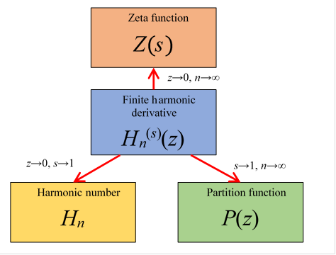
$$ \zeta(n) = -\frac{(2\pi)^n}{2\,n!}(-1)^{\frac{n}{2}+1}\,B_n. $$A new proof of 1 + 2 + 3 + ··· = −1/12 based on finite harmonic derivatives is given here:
This approach uses the finite harmonic derivative
$$ H_n^{(s)}(z) = \sum_{k=1}^n \frac{k^s}{k}e^{kz}, $$and recovers harmonic numbers, zeta values, and partition functions as limiting cases.
Quantizing this construction leads to the wave zeta function
$$ Z_q(s) = \sum_{k=1}^\infty \frac{1}{k^s}e^{kq}, $$ $$ \zeta_q(s) = \oint_C\frac{dz}{2\pi i(z-q)}\,Z_z(s), $$whose classical limit q→0 gives back ζ(s):
$$ \lim_{q\to0}\zeta_q(s) = \zeta(s). $$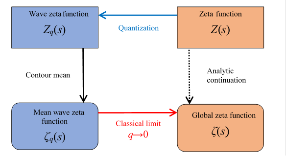
In this picture, analytic continuation can be viewed as a process of quantization, contour averaging, and then taking a classical limit.
© 2013, 2015 xseek-qm.net
広告