Derivation of the reflection integral equation of the zeta function by the complex analysis
Home > Quantum mechanics > Zeta function and Bernoulli numbers
2019/02/23
Published 2013/9/15
K. Sugiyama[1]
In this paper, we derive the reflection integral equation of the zeta function by the complex analysis.
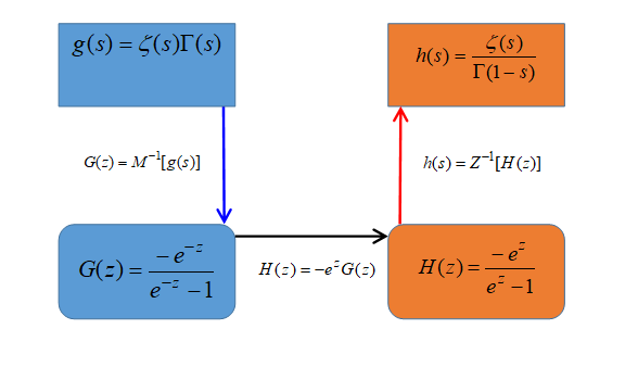
Figure 3-1: The framework of the method of derivation
Many researchers have attempted the proof of the Riemann hypothesis, but have not been successful. The proof of this Riemann hypothesis has been an important mathematical issue. In this paper, we attempt to derive the reflection integral equation by the complex analysis as preparation proving the Riemann hypothesis.
We obtain a generating function of the inverse Mellin-transform. We obtain a new generating function by multiplying the generating function with exponents and reversing the sign. We derive the reflection integral equation from the inverse Z-transform of the generating function.
We derive the Faulhaber’s formula, and Nörlund-Rice integral (or Rice's method) from the reflection integral equation.
CONTENTS
1.4 New derivation method of this paper
2 Confirmations of known results
3 Derivation of the reflection integral equation
3.1 The framework of the method of derivation
3.2 Derivation of the reflection integral equation from the inverse Mellin transform
6 Supplement 1: derivation of Faulhaber's formula.
6.1 Confirmations of known results (Part 2)
6.1.1 The Bernoulli polynomials
6.2 Derivation of Faulhaber's formula
6.2.1 Derivation of the summation equation of the Riemann zeta function
6.2.2 Derivation of the summation equation of the Hurwitz zeta function
6.2.3 Derivation of asymptotic expansion
6.2.4 Analytic continuation of asymptotic expansion.
6.2.5 Derivation of Faulhaber's formula
7 Supplement 2: Derivation of Nörlund-Rice integra.
7.1 Confirmations of known results (Part 3)
7.1.1 The Ramanujan master theorem
7.1.2 Woon's introduction of the continuous Bernoulli numbers
7.2 Derivation of Nörlund-Rice integral
7.2.1 Derivation of the reflection integral formula
7.2.2 Derivation of Nörlund-Rice integral
7.3 Consideration of the reflection integral equation
8.1 The table of the inverse Z-transform
1 Introduction
1.1 Issue
1.2 Importance of the issue
The proof of the Riemann hypothesis is one of the most important unsolved problems in mathematics.
For this reason, many researchers have attempted the proof of the Riemann hypothesis, but have not been successful. One of the methods proving Riemann hypothesis is interpreting the zeros of the zeta function as the eigenvalues of a certain operator. However, no one found the operator until now. We are able to consider the reflection integral equation as one of the operators. For this reason, the derivation of the reflection integral equation is an important issue.
1.3 Research trends so far
Leonhard Euler introduced the infinite series of the zeta function in 1737. Bernhard Riemann introduced the analytic continuation of the zeta function in 1859.
David Hilbert and George Polya[2] suggested that the zeros of the zeta function were probably eigenvalues of a certain operator around 1914. This conjecture is called Hilbert-Polya conjecture.
Zeev Rudnick and Peter Sarnak[3] are studying the distribution of zeros by random matrix theory in 1996. Shigenobu Kurokawa is studying the field with one element[4] around 1996. Alain Connes[5] showed the relation between noncommutative geometry and the Riemann hypothesis in 1998. Christopher Deninger[6] is studying the eigenvalue interpretation of the zeros in 1998.
1.4 New derivation method of this paper
We obtain a generating function of the inverse Mellin-transform. We obtain a new generating function by multiplying the generating function with exponents and reversing the sign. We derive the reflection integral equation from the inverse Z-transform of the generating function.
(The reflection integral equation)
|
|
(1.1) |
We derive the Faulhaber’s formula, and the Nörlund-Rice integral from the reflection integral equation.
(The Faulhaber’s formula)
|
|
(1.2) |
2 Confirmations of known results
In this chapter, we confirm the known results.
2.1 Cauchy’s residue theorem
Augustin-Louis Cauchy published the residue theorem[7] in 1831.
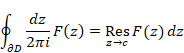
We suppose that a function F (z) has an isolated singularity c on a domain D inside of the simple closed curve ∂D and is holomorphic on both the domain D and the closed curve ∂D except for the isolated singularity. Then, we have the following formula.
(Residue theorem)
|
|
(2.1) |
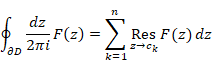
If a function F (z) has isolated singularities ck, we have the following formula.
(Residue theorem)
|
|
(2.2) |
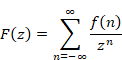
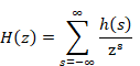
2.2 Hurewicz’s Z-transform
Witold Hurewicz [8] published the Z-transform in 1947. When a function F (z) is holomorphic over the domain D = {0<|z|< R}, we are able to transform the function to the series which converges uniformly in a wider sense over the domain.
(Z-transform)
|
|
(2.3) |
|
|
(2.4) |
|
|
(2.5) |
Therefore, when the minimum distance between an origin O and poles iR is R, we have the domain D of the Z-transform in the following figure. The white circles mean poles.
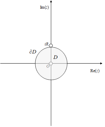
Figure 2-1: The domain of the Z-transform
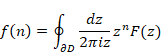
The inverse Z-transform is the contour integration along the circuit of integration ∂D circles the domain D.
(Inverse Z-transform)
|
|
(2.6) |
|
|
(2.7) |
2.3 The Mellin transform
Hjalmar Mellin[9] published the Mellin transform in 1904.
(The Mellin transform)
|
|
(2.8) |
|
|
(2.9) |
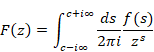
If a function f (s) is analytic in the strip S = {a < Re(s) < b}, and if it tends to zero uniformly as Im(s) → ±∞ for any real value c between a and b the following line integral converges absolutely.
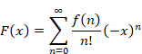
(The inverse Mellin transform)
|
|
(2.10) |
|
|
(2.11) |
|
|
(2.12) |
The real part of the strip S needs to be greater than the real part of all poles of the integrand. We show the strip S in the following figure. The white circles mean poles.
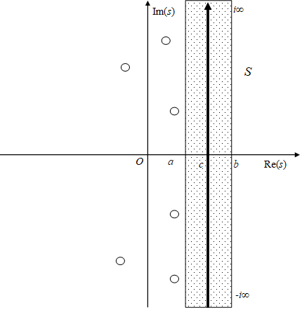
Figure 2-2: The strip S of the inverse Mellin transform
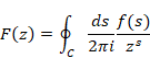
We define the inverse Mellin transform by the following contour integration.
(The inverse Mellin transform)
|
|
(2.13) |
|
|
(2.14) |
We suppose that the circuit of integration C circles around all poles of the integrand. For example, we suppose the circuit of integration C = CI + CR as follows. The white circles mean poles.
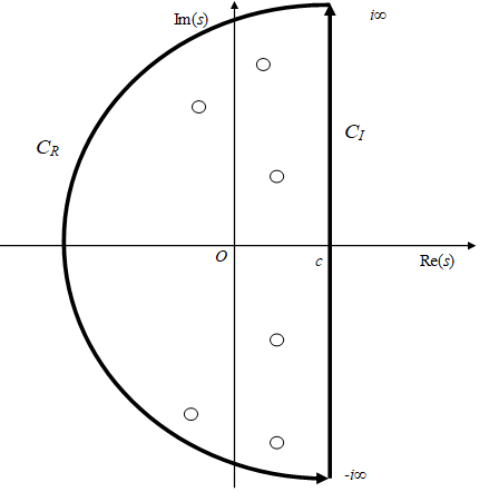
Figure 2-3: The inverse Mellin transform
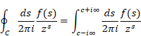
If the line integration of the path CR is zero, the contour integration of the circuit of integration C equals the line integration of the path CI. Then we have the following formula.
|
|
(2.15) |
2.4 Euler's gamma function
Leonhard Euler[10] introduced the gamma function as a generalization of the factorial in 1729.
(Gamma function)
|
|
(2.16) |
We get the following formula by replacing the variable x with (qx).
|
|
(2.17) |
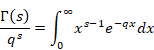
In the above formula, we replaced (dx) with (qdx).
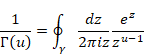
Hermann Hankel published the following integral representation[11] in 1863.
(The contour integration of gamma function)
|
|
(2.18) |
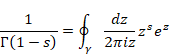
An integral path of gamma function is the path γ in the following figure. The white circles mean poles.
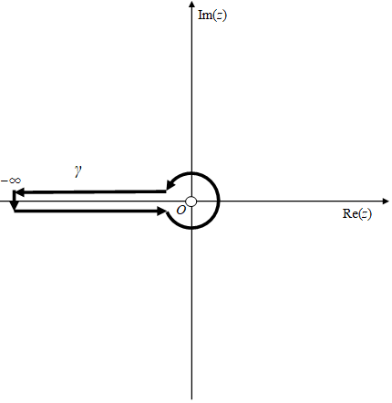
Figure 2-4: An integral path of the gamma function
We have the following formula for gamma function.
(Reflection formula of gamma function)
|
|
(2.19) |
The above formula is also called as Euler’s reflection formula.
2.5 Euler's beta function
Leonhard Euler introduced beta function in 1768 in his book[12].
(Beta function)
|
|
(2.20) |
We obtain the following reflection formula of the beta function from the reflection formula of the gamma function.
(The reflection formula of the Beta function)
|
|
(2.21) |
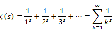
2.6 The Riemann zeta function
Leonhard Euler introduced the infinite series of the zeta function in 1737.
(The zeta function)
|
|
(2.22) |
Bernhard Riemann[13] expressed the zeta function by the gamma function in 1859.
(The zeta function)
|
|
(2.23) |
We interpret the above formula as the following Mellin transform.
(Mellin transform of zeta function)
|
|
(2.24) |
|
|
(2.25) |
|
|
(2.26) |
|
|
(2.27) |
We have the inverse Mellin transform as follows.
(Inverse Mellin transform of zeta function)
|
|
(2.28) |
|
|
(2.29) |
|
|
(2.30) |
|
|
(2.31) |
Bernhard Riemann introduced the analytic continuation of the zeta function in 1859.
(The analytic continuation of the zeta function)
|
|
(2.32) |
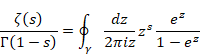
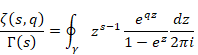
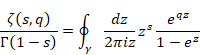
We interpret the above formula as the inverse Z-transform like the equation (2.7).
(Inverse Z-transform of zeta function)
|
|
(2.33) |
|
|
(2.34) |
|
|
(2.35) |
|
|
(2.36) |
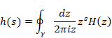
We show the integral path γ in the following figure. The white circles mean poles.
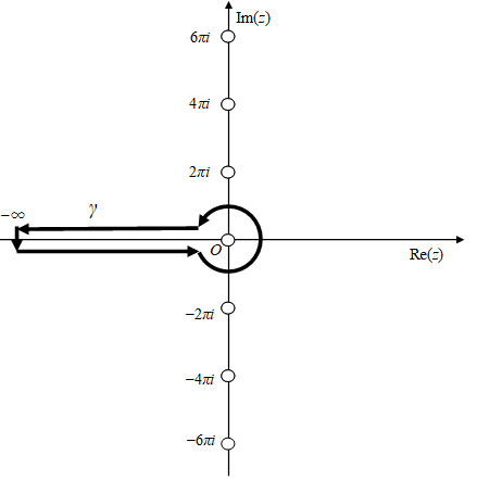
Figure 2-5: The integral path of the zeta function
We have the Z-transform of the zeta function as follows.
(Z-transform)
|
|
(2.37) |
|
|
(2.38) |
|
|
(2.39) |
|
|
(2.40) |
The generating functions of the Mellin transform and the Z-transform have the following relationship.
|
|
(2.41) |
|
|
(2.42) |
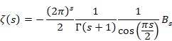
Riemann showed the following formula.
(Riemann’s reflection formula)
|
|
(2.43) |
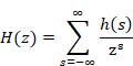
Riemann proposed the following conjecture in 1859.
(Riemann hypothesis)
Nontrivial zeros all have real part 1/2.
We express the examples of nontrivial zeros ρ1 and ρ2 in the following figure. The black circles are zeros, and the white circle means a pole.
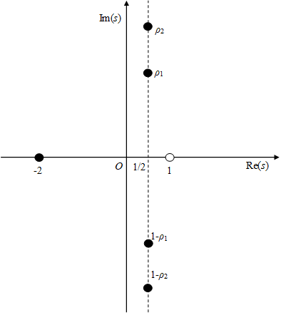
Figure 2-6: Nontrivial zeros of the zeta function
|
|
(2.44) |
|
|
(2.45) |
Since the proof of the Riemann hypothesis has not been successful, it has been an important mathematical issue.
3 Derivation of the reflection integral equation
3.1 The framework of the method of derivation
We have the following inverse Mellin transform of the zeta function.
|
|
(3.1) |
|
|
(3.2) |
|
|
(3.3) |
|
|
(3.4) |
We have the following inverse Z-transform of the zeta function.
|
|
(3.5) |
|
|
(3.6) |
|
|
(3.7) |
|
|
(3.8) |
The generating functions of the Mellin transform and Z-transform have the following relations.
|
|
(3.9) |
|
|
(3.10) |
We show the framework of the method of derivation in the following figure.

Figure 3-1: The framework of the method of derivation
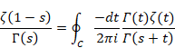
In this paper, we obtain the following equation.
(The reflection integral equation)
|
|
(3.11) |
This paper explains this derivation method.
3.2 Derivation of the reflection integral equation from the inverse Mellin transform
We have the following inverse Mellin transform of the zeta function.
|
|
(3.12) |
|
|
(3.13) |
|
|
(3.14) |
|
|
(3.15) |
In the inverse Mellin transform, the circuit of the integration C needs to circle around all poles of the integrand. Then, we adopt the following circuit of integration C. The white circles mean poles.
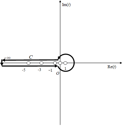
Figure 3-2: The integral path of the inverse Mellin transform
On the other hand, we have the following inverse Z-transform of the zeta function.
(Inverse Z-transform)
|
|
(3.16) |
|
|
(3.17) |
|
|
(3.18) |
|
|
(3.19) |
We show the integral path γ in the following figure. The white circles mean poles.
Figure 3-3: The integral path of the zeta function
By using the equation (2.41), we deform the inverse Z-transform as follows.
|
|
(3.20) |
We replace the variable s with the variable (1-s) in the above formula.
|
|
(3.21) |
We obtain the following equation by substituting the inverse Mellin transform for the function G (z).
|
|
(3.22) |
In order to take the integral of the above equation with the respect to the variable z, we deform the above equation.
|
|
(3.23) |
We apply the following formula to the above equation.
(Contour integration of gamma function)
|
|
(3.24) |
Then, we get the following equation.
|
|
(3.25) |
|
|
(3.26) |
|
|
(3.27) |
Here, we simplify the above equation by using the following beta function (2.20).
|
|
(3.28) |
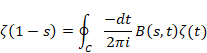
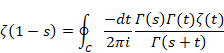
As the result, we obtain the following equation.
(Reflection integral equation)
|
|
(3.29) |
We show the integral path C in the following figure. The white circles mean poles.

Figure 3-4: The integral path of the reflection integral equation of the zeta function
4 Conclusion
We obtained the following result in this paper.
- We derived the reflection integral equation of the zeta function.
5 Future issues
We have the following future issues.
- To derive Faulhaber’s formula
- To derive Nörlund-Rice integral
- To study the eigenvalues of the integral equation
- To study the relation between the generating function of Z-transform and zeros
6 Supplement 1: derivation of Faulhaber's formula
In the supplement, after we confirm the known results, we derive the following formulas.
- Faulhaber’s formula
- Nörlund-Rice integral
6.1 Confirmations of known results (Part 2)
In this section, we confirm the known results.
6.1.1 The Bernoulli polynomials
We define the Bernoulli polynomials as follows.
(The Bernoulli polynomials)
|
|
(6.1) |
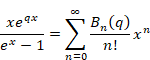
The above series does not converge over the whole domain. The radius of convergence is 2π because the minimum distance between the origin and poles of the generating function is 2π.
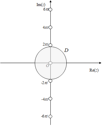
Figure 6-1: The radius of convergence of the Bernoulli polynomials
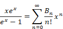
6.1.2 The Bernoulli numbers
Jakob Bernoulli introduced the Bernoulli numbers in 1713 in his book[14].
(The Bernoulli numbers)
|
|
(6.2) |
We have the following formula for the even positive integer n.
(The reflection formula of the Bernoulli numbers)
|
|
(6.3) |
According to Vich’s book[15], we have the following Z-transform.
(The Z-transform of the Bernoulli numbers)
|
|
(6.4) |
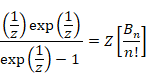
In this paper, we use the following Z-transform.
(The Z-transform of the Bernoulli numbers)
|
|
(6.5) |
|
|
(6.6) |
|
|
(6.7) |
|
|
(6.8) |
On the other hand, we have the Z-transform of the zeta function as follows.
(Z-transform of the zeta function)
|
|
(6.9) |
|
|
(6.10) |
|
|
(6.11) |
|
|
(6.12) |
Therefore, we have the following equation.
|
|
(6.13) |
We obtain the following formula by replacing the variable s with the negative integer -n.
(The formula of the Bernoulli numbers)
|
|
(6.14) |
Traditionally, we consider that the Bernoulli numbers are discrete. I consider that the Bernoulli numbers are continuous. We call the continual Bernoulli numbers the Bernoulli function. I interpret that the Bernoulli function is the following different representation of the zeta function.
|
|
(6.15) |
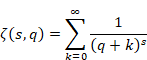
6.1.3 Hurwitz zeta function
Adolf Hurwitz[16] introduced the following zeta function in 1882.
(The Hurwitz zeta function)
|
|
(6.16) |
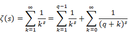
We have the following relationship between the Hurwitz zeta function and the Riemann zeta function.
|
|
(6.17) |
|
|
(6.18) |
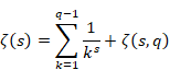
The Hurwitz zeta function becomes the Riemann zeta function when q is equal to one.
|
|
(6.19) |
We express the Hurwitz zeta function by the gamma function.
(The Hurwitz zeta function)
|
|
(6.20) |
We interpret the above formula as the following Mellin transform.
(The Mellin transform)
|
|
(6.21) |
|
|
(6.22) |
|
|
(6.23) |
|
|
(6.24) |
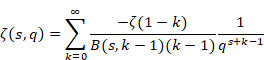
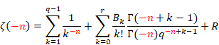
We have the following analytic continuation of the Hurwitz zeta function.
(The analytic continuation of the Hurwitz zeta function)
|
|
(6.25) |
We interpret the above formula as the following inverse Z-transform.
(The inverse Z-transform)
|
|
(6.26) |
|
|
(6.27) |
|
|
(6.28) |
|
|
(6.29) |
We have the following equation for the natural number n.
(Formula of Bernoulli polynomials)
|
|
(6.30) |
6.1.4 Euler-Maclaurin formula
Euler[17] discovered the following formula in 1738. Maclaurin[18] have also discovered the same formula in 1742 independently.
(The Euler-Maclaurin formula)
|
|
(6.31) |
|
|
(6.32) |
|
|
(6.33) |

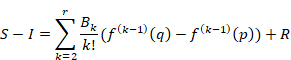
In the above formula, the variable R is an error term.
6.1.5 Asymptotic expansion
Euler[19] calculated the value of the zeta function by Euler-Maclaurin formula in 1755.
(The asymptotic expansion of the zeta function)
|
|
(6.34) |
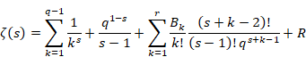
In the above formula, the variable R is an error term. The detail method to derive the above formula is shown in the book[20] by Edwards in 1974.
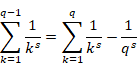
Here, we use the following equation.
|
|
(6.35) |
Then, we obtain the following formula.
(The asymptotic expansion of the zeta function)
|
|
(6.36) |
6.1.6 Faulhaber's formula
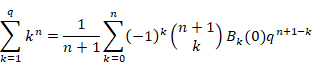
Johann Faulhaber[21] published the formula of the sum of powers in 1631. We have the following formula for the natural number n.
(Faulhaber’s formula)
|
|
(6.37) |
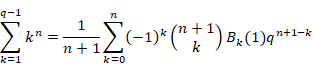
We express the above formula by using the Bernoulli polynomial Bk (1).
(Faulhaber’s formula)
|
|
(6.38) |
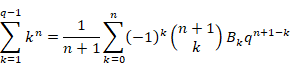
In this paper, we express the above formula by the Bernoulli numbers Bk as follows.
(Faulhaber’s formula)
|
|
(6.39) |
6.2 Derivation of Faulhaber's formula
In order to derive Faulhaber's formula, we derive the following formulas.
- The summation equation of the Riemann zeta function
- The summation equation of the Hurwitz zeta function
- The asymptotic expansion of the Riemann zeta function
6.2.1 Derivation of the summation equation of the Riemann zeta function
We derive the summation equation of the Riemann zeta function.
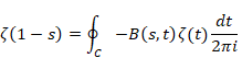
We have the following reflection integral equation.
(The reflection integral equation)
|
|
(6.40) |
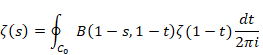
We replace the variable s with (1-s) and we replace the variable t with (1-t) in the above equation.
(The reflection integral equation)
|
|
(6.41) |
We show the integral path C0 in the following figure. The white circles mean poles.
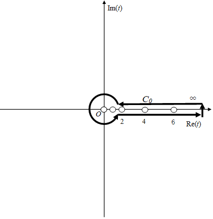
Figure 6-2: The integral path of the reflection integral equation
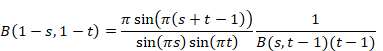
We substitute the following formula into the above equation.
(Reflection formula of Beta function)
|
|
(6.42) |
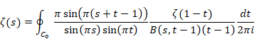
Then, we obtain the following formula.
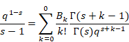
|
|
(6.43) |
We take the integral of the above integration by the residue theorem.
|
|
(6.44) |
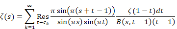
Here, ck is the k-th pole. The singularities are 0, 1, 2, 4, 6, …
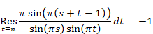
We have the following equation for integer n.
|
|
(6.45) |
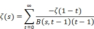
We express derive the following equation since the all singularities are integers and the value of the zeta function ζ (1-t) is zero at t = 3, 5, 7, ∙∙∙.
(The summation equation)
|
|
(6.46) |
We are not able to calculate by the above equation because it diverges. In order to solve the problem, we derive the summation equation of the Hurwitz zeta function in the next section.
6.2.2 Derivation of the summation equation of the Hurwitz zeta function
In this section, we derive the summation equation of the Hurwitz zeta function.
We have the following Hurwitz zeta function.
(The Hurwitz zeta function)
|
|
(6.47) |
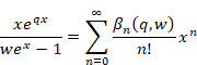
We express the above formula by the generating function of the Mellin transform.
|
|
(6.48) |
We can obtain the following equation by deforming the above formula.
|
|
(6.49) |
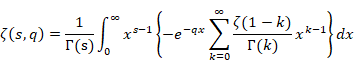
We obtain the following equation by substituting the Z-transform for the function H (x) of the above equation.
|
|
(6.50) |
|
|
(6.51) |
The Z-transform converges over the domain D. Therefore, we are able to change the order of the integration and the summation over the domain.
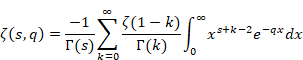
In order to take the integral of the above equation with respect to the variable x, we deform the above equation as follows.
|
|
(6.52) |
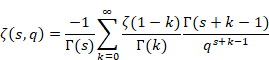
We apply the following equation (2.17) of gamma function to the above equation.
|
|
(6.53) |
As the result, we obtain the following equation.
|
|
(6.54) |
Here, we simplify the above equation by using the following beta function (2.20).
|
|
(6.55) |
As the result, we obtain the following equation.
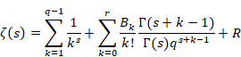
(The summation equation of the Hurwitz zeta function)
|
|
(6.56) |
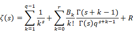
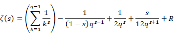
The solution of the above equation reaches an infinite value because the convergent radius of a “definitional series of the Bernoulli function” is 2π. Therefore, we change the upper limit of the summation to a variable r which depends on the variable q.
(The summation equation of the Hurwitz zeta function)
|
|
(6.57) |
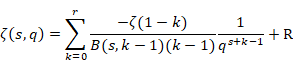
Here, R is an error term.
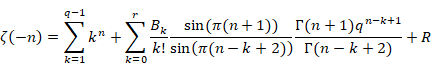
6.2.3 Derivation of asymptotic expansion
In this section, we derive the asymptotic expansion of the zeta function, (6.36).
We have the following relation between the Riemann and Hurwitz zeta function.
|
|
(6.58) |
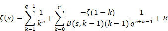
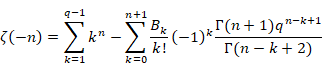
Therefore, we are able to express the summation equation of the Riemann zeta function as follows.
(The summation equation)
|
|
(6.59) |
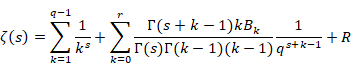
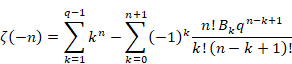
We obtain the following equation by replacing the beta function to the gamma function.
|
|
(6.60) |

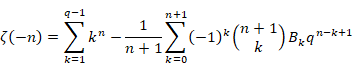
We deform the above equation by the formula of the Bernoulli polynomials as follows.
|
|
(6.61) |
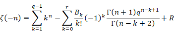
We obtain the following asymptotic expansion of the zeta function by deforming the above equation.
(The asymptotic expansion of the zeta function)
|
|
(6.62) |
6.2.4 Analytic continuation of asymptotic expansion
The following expression is known as the expression of zeta function for -3<Re(s).
|
|
(6.63) |
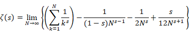
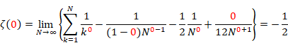
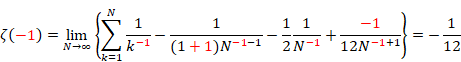
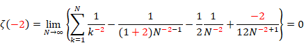
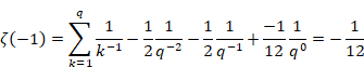
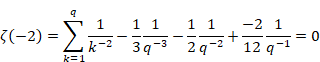
We are able to calculate the value of the zeta function of s=0, -1, -2 by the above formula.
|
|
(6.64) |
|
|
(6.65) |
|
|
(6.66) |
We can derive the expression (6.62) from the analytic continuation of the asymptotic expansion of the zeta function. In this section, we derive the expression (6.62).
We have the asymptotic expansion of the zeta function (6.36) as follows.
The asymptotic expansion of the zeta function)
|
|
(6.67) |
We focus the following part of the above formula.
|
|
(6.68) |
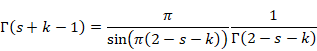
Here, we use reflection formula of gamma function (2.19).
|
|
(6.69) |
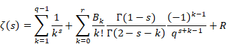
Then, we have the following equations.
|
|
(6.70) |
|
|
(6.71) |
Therefore, we obtain the following formula.
|
|
(6.72) |
Here we have the following equation for the integer k.
|
|
(6.73) |
Therefore, we obtain the following equation.
|
|
(6.74) |
We obtain the following analytic continuation of asymptotic expansion of the zeta function by substituting the above equation(6.74) into the equation (6.67).
(The analytic continuation of asymptotic expansion of the zeta function)
|
|
(6.75) |
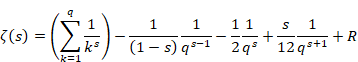
We expand the above formula by r = 3.
|
|
(6.76) |
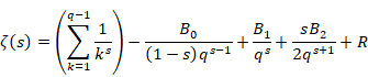
Here we substitute the values into the Bernoulli numbers in the above formula.
|
|
(6.77) |
On the other hand, we are able to separate the first term as follows.
|
|
(6.78) |
Therefore, we obtain the following formula.
|
|
(6.79) |
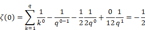
We are able to calculate the value of the zeta function of s=0, -1, -2 by the above formula.
|
|
(6.80) |
|
|
(6.81) |
|
|
(6.82) |
The variable q comes from the following formula.
|
|
(6.83) |
|
|
(6.84) |
Therefore, the variable q of the formula (6.75) is not infinite but finite.
6.2.5 Derivation of Faulhaber's formula
In this section, we derive Faulhaber's formula.
We have the asymptotic expansion of the zeta function (6.36) as follows.
(The asymptotic expansion of the zeta function)
|
|
(6.85) |
We replace the variable s with (-n) in the above equation.
|
|
(6.86) |
We deform the above equation by Euler’s reflection formula as follows.
|
|
(6.87) |
We have the following equation for the integer k.
|
|
(6.88) |
Therefore, we obtain the following equation.
|
|
(6.89) |
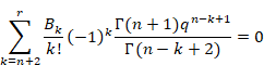
We have the following equation for the natural number n and the integer k > n+1.
|
|
(6.90) |
Therefore, we obtain the following equation.
|
|
(6.91) |
We remove the error term R and change the upper limit of summation to n+1 of the equation (6.89) because the values of the all terms at k > n+1 are zero.
|
|
(6.92) |
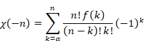
We express the following equation by using the factorial.
|
|
(6.93) |
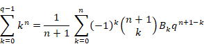
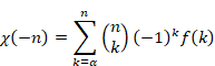
We express the following equation by using the binomial coefficient.
|
|
(6.94) |
We deform the above equation by the formula of the Bernoulli polynomials as follows.
|
|
(6.95) |

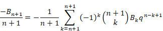
We have the following equation for the natural number n and the integer k = n+1.
|
|
(6.96) |
According to the above result, we obtain the following equation.
|
|
(6.97) |
Therefore, we obtain the following Faulhaber's formula by deforming the formula (6.95).
(Faulhaber's formula)
|
|
(6.98) |
The above formula was a formula to be derived in this section.
7 Supplement 2: Derivation of Nörlund-Rice integra
7.1 Confirmations of known results (Part 3)
In this section, we confirm the known results.
7.1.1 The Ramanujan master theorem
Srinivasa Ramanujan obtained the following theorem[22] for real number x and complex number s about 1910.
(The Ramanujan master theorem)
|
|
(7.1) |
|
|
(7.2) |
We have the above equations for the following Bernoulli numbers and the zeta function.
|
|
(7.3) |
|
|
(7.4) |
|
|
(7.5) |
This theorem suggests that the following relation.
|
|
(7.6) |
7.1.2 Woon's introduction of the continuous Bernoulli numbers
S. C. Woon[23] introduced the continuous Bernoulli numbers in 1997.
We have the following formula for the natural number n.
(Formula of the Bernoulli numbers)
|
|
(7.7) |
Woon proposed the following formula for the complex number s.
(The formula of the Bernoulli function)
|
|
(7.8) |
In this paper, we use the following notation for the Bernoulli function based on the notation for the Bernoulli numbers.
(The formula of the Bernoulli function)
|
|
(7.9) |
We obtain the following equation by substituting the above formula into Riemann’s reflection formula.
|
|
(7.10) |
We obtain the following equation by deforming the above formula.
(The reflection formula of the Bernoulli function)
|
|
(7.11) |
The above formula becomes the following formula for the even positive integer s.
|
|
(7.12) |
The above formula is equal to the following formula for the even positive integer n.
(The reflection formula of the Bernoulli numbers)
|
|
(7.13) |
The above result suggests that the validity of the formula of the Bernoulli function.
7.1.3 Nörlund-Rice integral
Niels Erik Nörlund[24] published the Nörlund-Rice integral (or Rice's method) in 1924.
(Nörlund-Rice integral)
|
|
(7.14) |
Here, the path C circles around poles c, …, and n for positive integer c. B (x, y) is Euler’s beta function.
Philippe Flajolet[25] published the Poisson-Mellin-Newton cycle in 1985 for the Nörlund-Rice integral.
(Poisson-Mellin-Newton cycle)
|
|
(7.15) |
|
|
(7.16) |
|
|
(7.17) |
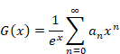
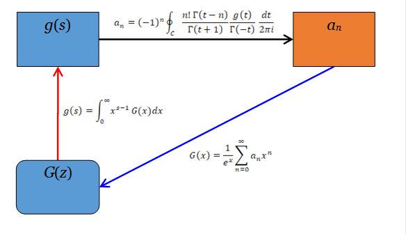
Figure 7-1: The Poisson-Mellin-Newton cycle
7.2 Derivation of Nörlund-Rice integral
7.2.1 Derivation of the reflection integral formula
We define a new function H (z).
|
|
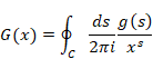
(7.18) |
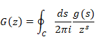
We obtain a new function g(s) from the Mellin transform of the function G(z).
|
|
(7.19) |
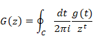
We have the following inverse Mellin transform.
|
|
(7.20) |
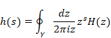
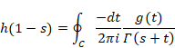
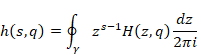
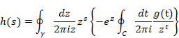
We obtain a new function h(s) from the inverse Z-transform of the function H(z).
|
|
(7.21) |
We show the relation of the above functions in the following figure.
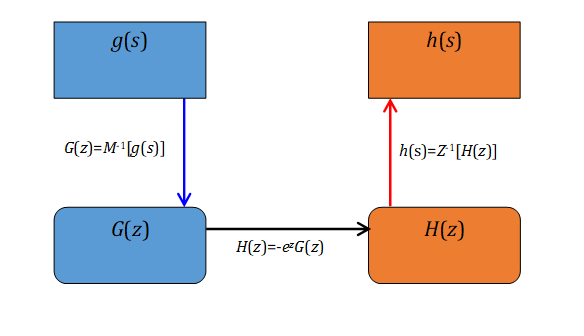
Figure 7-2: The inverse Mellin transform and the inverse Z-transform
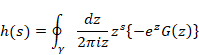
We have the following formula of the inverse Z-transform from the equation (2.7).
|
|
(7.22) |
We deform the formula of the inverse Z-transform as follows.
|
|
(7.23) |
We substitute the inverse Mellin transform for the function G (x) of the above formula.
|
|
(7.24) |
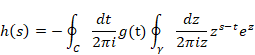
In order to take the integral of the above formula with respect to the variable z, we deform the above formula.
|
|
(7.25) |
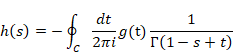
We apply the following contour integration of the gamma function to the above equation.
|
|
(7.26) |
As the result, we obtain the following equation.
|
|
(7.27) |
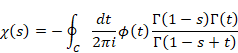
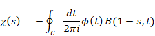
We define the new
functions ![]() and χ (s) as follows.
and χ (s) as follows.
|
|
(7.28) |
|
|
(7.29) |
Then, we are able to deform the formula (7.27) as follows.
|
|
(7.30) |
We express the above formula by Euler’s Beta function as follows.
(The reflection integral formula)
|
|
(7.31) |
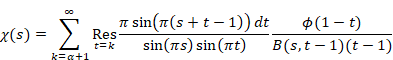
7.2.2 Derivation of Nörlund-Rice integral
In this section, we derive Nörlund-Rice integral.
We obtain the following summation formula by adopting residue theorem to the
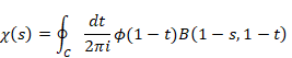
We replace the variable t with (1-t) in the reflection integral formula (7.31).
(The reflection integral equation)
|
|
(7.32) |
We show the integral path C in the following figure. The white circles mean poles.
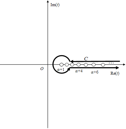
Figure 7-3: The integral path of the reflection integral equation
Here, α is an integer number, 0 ≤ α.
We substitute the following formula into the above equation.
(Reflection formula of Beta function)
|
|
(7.33) |
Then, we obtain the following formula.
|
|
(7.34) |
We take the integral of the above integration by the residue theorem.
|
|
(7.35) |
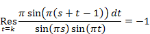
Here, singularities are α+1, α+2, α+3,….
We have the following equation for integer k.
|
|
(7.36) |
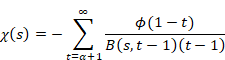
Therefore, we obtain the following equation.
(Summation equation)
|
|
(7.37) |
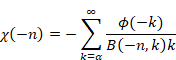
We replace the variable s with (-n), and we replace the variable t with (k+1) in the above equation.
|
|
(7.38) |
Here, we define a new function f(k).
|
|
(7.39) |
We express the formula by the function f(k).
|
|
(7.40) |
We replace the gamma function for the beta function.
|
|
(7.41) |
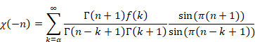
We obtain the following formula by using Euler’s reflection formula.
|
|
(7.42) |
We have the following equation for the integer k.
|
|
(7.43) |
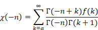
Therefore, we obtain the following formula.
|
|
(7.44) |

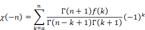
We have the following equation for the natural number n and the integer k > n.
|
|
(7.45) |
We change the variable m to n, because the values of the all terms at k > n are zero.
|
|
(7.46) |
We express the following equation by using the factorial.
|
|
(7.47) |
We express the following equation by using the binomial coefficient.
|
|
(7.48) |
On the other hand, we have the following reflection integral formula.
(Reflection integral formula)
|
|
(7.49) |
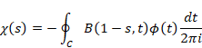
We replace the variable s with (-n), and we replace the variable t to (-t) in the above equation.
|
|
(7.50) |
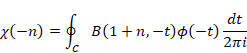
Here, we define a new function f (t).
|
|
(7.51) |
Then, we obtain the following equation.
|
|
(7.52) |
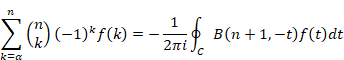
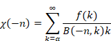
We obtain the following equation form the equation (7.48) and (7.52).
(The Nörlund-Rice integral)
|
|
(7.53) |
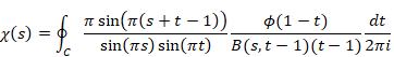
7.3 Consideration of the reflection integral equation
We show the reflection integral formula as follows.
(The reflection integral formula)
|
|
(7.54) |
In the above equation, we suppose the following condition.
|
|
(7.55) |
Then, we obtain the following relation.
|
|
(7.56) |
Therefore, the following two equations are equivalent.
|
|
(7.57) |
|
|
(7.58) |
8 Appendix
8.1 The table of the inverse Z-transform
We show the table of the inverse Z-transform as follows.
Table 8‑1:Inverse Z-transform
|
# |
|
|
Num. |
|
1 |
|
|
(8.1) |
|
2 |
|
|
(8.2) |
|
3 |
|
|
(8.3) |
|
4 |
|
|
(8.4) |
|
5 |
|
|
(8.5) |
|
6 |
|
|
(8.6) |
We show the above functions as follows.
(The Riemann zeta function)
|
|
(8.7) |
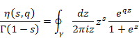
(Dirichlet[26] eta function)
|
|
(8.8) |
(Hurwitz zeta function)
|
|
(8.9) |
(Hurwitz eta function)
|
|
(8.10) |
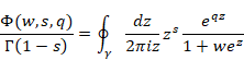
(Lerch transcendent[27])
|
|
(8.11) |
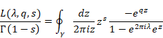
(Lerch zeta function)
|
|
(8.12) |
The formulas of the polynomials are shown below.
|
|
(8.13) |
|
|
(8.14) |
|
|
(8.15) |
|
|
(8.16) |
|
|
(8.17) |
We show the definition of the polynomials as follows.
(The Bernoulli polynomials)
|
|
(8.18) |
(The Euler polynomials)
|
|
(8.19) |
(The Apostol-Bernoulli polynomials [28])
|
|
(8.20) |