Derivation of the reflection integral equation of the zeta function by the quaternionic analysis
Home > Quantum mechanics > Zeta function and Bernoulli numbers
2019/02/23
Published 2014/5/18
K. Sugiyama[1]
We derive the reflection integral equation of the zeta function by the quaternionic analysis.
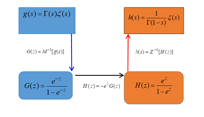
Figure 3.1: The framework of the method of derivation
Many researchers have attempted proof of the Riemann hypothesis, but they have not been successful. The proof of this Riemann hypothesis has been an important mathematical issue. In this paper, we attempt to derive the reflection integral equation from the quaternionic analysis as preparation proving the Riemann hypothesis.
We obtain a generating function of the inverse Mellin-transform. We obtain new generating function by multiplying the generating function with exponents and reversing the sign. We derive the reflection integral equation from inverse Z-transform of the generating function.
CONTENTS
1.4 New derivation method of this paper
2 Confirmations of known results
3 Derivation of the reflection integral equation
3.1 The framework of the method of derivation
3.2 Derivation of the reflection integral equation from the inverse Mellin transform
1 Introduction
1.1 Issue
1.2 Importance of the issue
Proof of the Riemann hypothesis is one of the most important unsolved problems in mathematics.
For this reason, many mathematicians have tried the proof of the Riemann hypothesis. However, those trials were not successful. One of the methods proving Riemann hypothesis is interpreting the zeros of the zeta function as the eigenvalues of a certain operator. However, no one found the operator until now. We are able to consider the reflection integral equation as the one of the operators. For this reason, derivation of the reflection integral equation is an important issue.
1.3 Research trends so far
Leonhard Euler introduced the zeta function in 1737. Bernhard Riemann expanded the argument of the function to the complex number in 1859.
David Hilbert and George Polya[2] suggested that the zeros of the function were probably eigenvalues of a certain operator around 1914. This conjecture is called Hilbert-Polya conjecture.
Zeev Rudnick and Peter Sarnak[3] are studying the distribution of zeros by random matrix theory in 1996. Shigenobu Kurokawa is studying the field with one element[4] around 1996. Alain Connes[5] showed the relation between noncommutative geometry and the Riemann hypothesis in 1998. Christopher Deninger[6] is studying the eigenvalue interpretation of the zeros in 1998.
1.4 New derivation method of this paper
We obtain a generating function of the inverse Mellin-transform. We obtain new generating function by multiplying the generating function with exponents and reversing the sign. We derive the reflection integral equation from inverse Z-transform of the generating function.
(Reflection integral equation of quaternion)
|
|
(1.1) |
The variable u is a new unit quaternion which is constructed by unit quaternions i, j, and k.
|
|
(1.2) |
|
|
(1.3) |
2 Confirmations of known results
In this chapter, we confirm known results.
2.1 The quaternion
Euler used the complex number in about 1748.
|
|
(2.1) |
William Rowan Hamilton[7] published the quaternion in 1843.
|
|
(2.2) |
We define the quaternion as follows.
|
|
(2.3) |
|
|
(2.4) |
We define the order of the division of the quaternions as follows.
(The order of the division of the quaternions)
|
|
(2.5) |
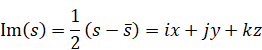
We define the quaternion conjugate as follows.
|
|
(2.6) |
We define the quaternionic function as follows.
|
|
(2.7) |
We define the absolute square as follows.
|
|
(2.8) |
In this paper, we define the following symbols.
|
|
(2.9) |
|
|
(2.10) |
2.2 The quaternionic analysis
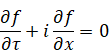
Augustin-Louis Cauchy [8] introduced the following equation for the complex analysis in 1814. Riemann[9] used this equation for the complex analysis in 1851.
(Cauchy - Riemann differential equation)
|
|
(2.11) |
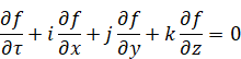
Karl Rudolf Fueter [10] introduced the following equation as the analogue of Cauchy - Riemann equation for the quaternionic analysis in 1934.
(Cauchy - Riemann - Fueter differential equation)
|
|
(2.12) |
Cauchy introduced the following integral formula.
(Cauchy's integral formula)
|
|
(2.13) |
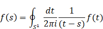
Here, S1 is the contour path.
Fueter introduced the following formula as the analogue of Cauchy's integral formula.
(Cauchy - Fueter's integral formula)
|
|
(2.14) |
Here S 3 is the three-dimensional closed surface. We define Dq as follows.
|
|
(2.15) |
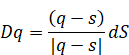
Here dS is the volume element on the three-dimensional closed surface S 3.
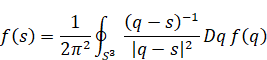
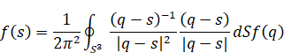
We obtain the following formula by substituting the above formula to the integral formula.
|
|
(2.16) |
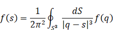
|
|
(2.17) |
The detail of the quaternionic analysis described in Sudbery’s paper[11] in 1979.
The above formula has an absolute value of the quaternion. In this paper, we introduce the following new formula that does not have the absolute value of the quaternion.
(Cauchy's integral formula for quaternions)
|
|
(2.18) |
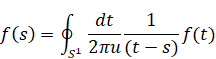
Here, S1 is the integral path in quaternionic space.
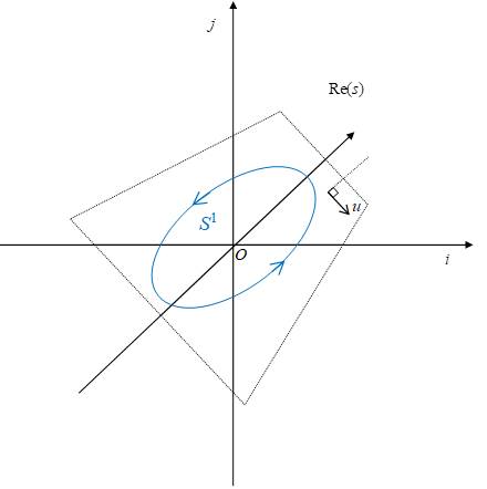
Figure 2.1: The integral path S1 in quaternionic space
We call the plane that contain the integral path S1 unit quaternion plane. Though quaternion is noncommutative, the quaternion on the unit quaternion plane is commutative. Therefore, we can ignore the noncommutativity of the quaternion.
The variable u is a new unit quaternion which is constructed by unit quaternions i, j, and k.
|
|
(2.19) |
|
|
(2.20) |
We can express any unit quaternion q on the unit quaternion plane as follows.
|
|
(2.21) |
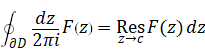
2.3 Cauchy’s residue theorem
Augustin-Louis Cauchy published the residue theorem[12] in 1831.
We suppose that a function F (z) has an isolated singularity c on a domain D. Then, we have the following formula for the simple closed curve ∂D circles round the domain D.
(The residue theorem)
|
|
(2.22) |
We define the residue theorem for the quaternion as follows.
(The residue theorem for the quaternion)
|
|
(2.23) |
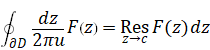
Here, the variable u is a unit quaternion.
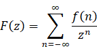
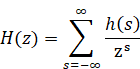
2.4 Hurewicz’s Z-transform
Witold Hurewicz [13] published Z-transform in 1947. When the function F (z) is holomorphic over the domain D = {0 <|z|< R}, we are able to transform the function to the series which converges uniformly in a wider sense over the domain.
(Z-transform)
|
|
(2.24) |
|
|
(2.25) |
|
|
(2.26) |
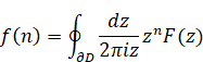
We define the inverse Z-transform as follows.
(Inverse Z-transform)
|
|
(2.27) |
|
|
(2.28) |
We define the inverse Z-transform of the quaternion as follows.
(Inverse Z-transform of the quaternion)
|
|
(2.29) |
|
|
(2.30) |
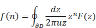
Here, the variable u is a unit quaternion.
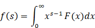
2.5 The Mellin transform
Hjalmar Mellin[14] published the Mellin transform in 1904.
(The Mellin transform)
|
|
(2.31) |
|
|
(2.32) |
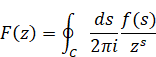
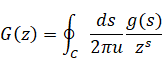
We define the inverse Mellin transform by the following contour integration.
(The inverse Mellin transform)
|
|
(2.33) |
|
|
(2.34) |
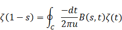
On the other hand, we define the inverse Mellin transform of quaternion by the following contour integration.
(The inverse Mellin transform of quaternion)
|
|
(2.35) |
|
|
(2.36) |
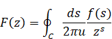
Here C is the integral path in quaternion space. The variable u is a unit quaternion.
The integral path circles around all poles of the integrand. For example, we suppose the integral path S1 as follows. The white circles mean poles.

Figure 2.2: The integral path C in the quaternionic space
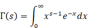
2.6 Euler's gamma function
Leonhard Euler[15] introduced the gamma function as a generalization of the factorial in 1729.
(Definitional integral formula of the gamma function)
|
|
(2.37) |
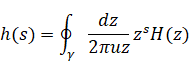
We introduced the integral representation of the gamma function.
(Contour integration of gamma function)
|
|
(2.38) |
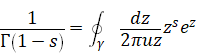
Here, the variable u is a unit quaternion.
The integral path γ is shown in the following figure. The white circles mean poles.
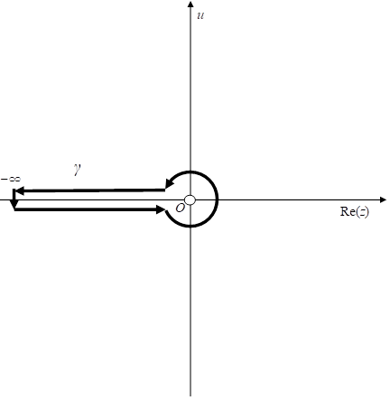
Figure 2-3: The integral path of the gamma function
2.7 Euler's beta function
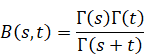
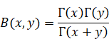
Leonhard Euler introduced the beta function in 1768 in his book[16]. We express the Beta function by using the gamma functions.
(Definitional formula of the beta function)
|
|
(2.39) |
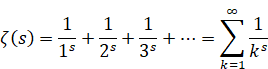
2.8 Riemann zeta function
Bernhard Riemann[17] introduced the zeta function in 1859.
(The zeta function)
|
|
(2.40) |
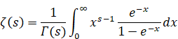
We express the zeta function by the gamma function as follows.
(The zeta function)
|
|
(2.41) |
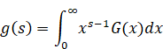
We interpret the above formula as the following Mellin transform.
(The Mellin transform)
|
|
(2.42) |
|
|
(2.43) |
|
|
(2.44) |
|
|
(2.45) |
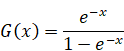
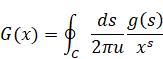
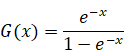
We have the inverse Mellin transform of the function as follows.
(The inverse Mellin transform)
|
|
(2.46) |
|
|
(2.47) |
|
|
(2.48) |
|
|
(2.49) |
The variable u is a unit quaternion.
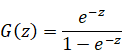
We have the analytic continuation of the zeta function as follows.
(The analytic continuation of the zeta function)
|
|
(2.50) |
We interpret the above formula as the following the inverse Z-transform.
(Inverse Z-transform)
|
|
(2.51) |
|
|
(2.52) |
|
|
(2.53) |
|
|
(2.54) |
We show the closed surface γ3 in the following figure. The white circles mean poles.
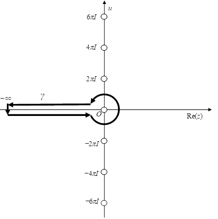
Figure 2.4: The integral path of the zeta function
We have the Z-transform of the function as follows.
(The Z-transform)
|
|
(2.55) |
|
|
(2.56) |
|
|
(2.57) |
|
|
(2.58) |
The generating functions of the Mellin transform and Z-transform have the following relationship.
|
|
(2.59) |
|
|
(2.60) |
3 Derivation of the reflection integral equation
3.1 The framework of the method of derivation
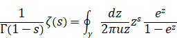
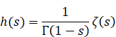
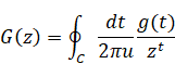
We have the inverse Mellin transform of zeta function as follows.
|
|
(3.1) |
|
|
(3.2) |
|
|
(3.3) |
|
|
(3.4) |
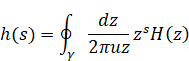
We have the inverse Z-transform of the function as follows.
|
|
(3.5) |
|
|
(3.6) |
|
|
(3.7) |
|
|
(3.8) |
The generating functions of the Mellin transform and Z-transform have the following relationships.
|
|
(3.9) |
|
|
(3.10) |
We show the framework of the method of derivation in the following figure.
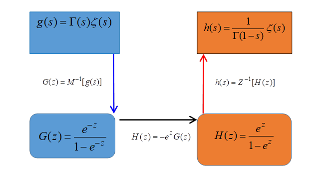
Figure 3.1: The framework of the method of derivation
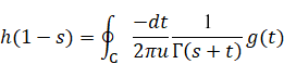
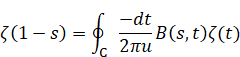
We get the reflection integral equation by the above framework.
(Reflection integral equation)
|
|
(3.11) |
This paper explains this derivation method.
3.2 Derivation of the reflection integral equation from the inverse Mellin transform
We have the inverse Mellin transform of the zeta function as follows.
|
|
(3.12) |
|
|
(3.13) |
|
|
(3.14) |
|
|
(3.15) |
The three-dimensional closed surface S3 of the inverse Mellin transform needs to circle around all poles of the integrand. Then we adopt the closed surface S3 as follows. The white circles mean poles.
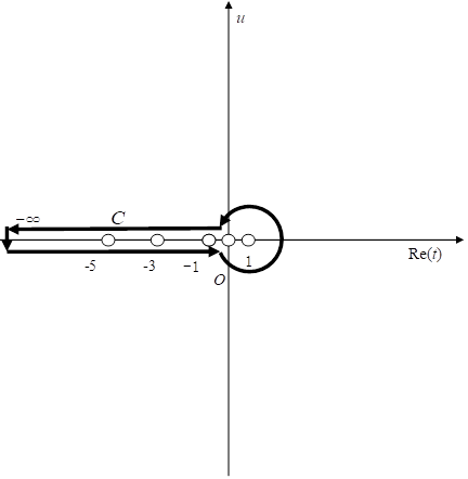
Figure 3.2: The integral path of the inverse Mellin transform
On the other hand, we have the inverse Z-transform of the function as follows.
(Inverse Z-transform)
|
|
(3.16) |
|
|
(3.17) |
|
|
(3.18) |
|
|
(3.19) |
We show the integral path in the following figure. The white circles mean poles.
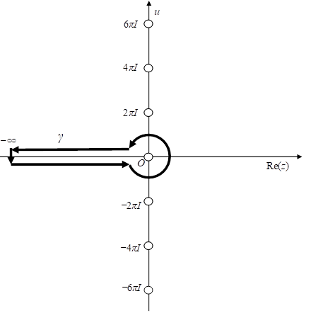
Figure 3.3: The integral path of the zeta function
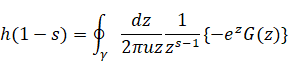
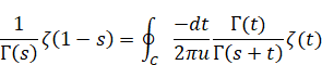
We deform the equation of the inverse Z-transform as follows.
|
|
(3.20) |
We replace s to 1-s as follows.
|
|
(3.21) |
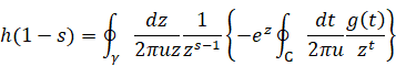
We obtain the following equation by substituting the equation of the inverse Mellin transform.
|
|
(3.22) |
The quaternion on the unit quaternion plane is commutative. We can ignore the noncommutativity of the quaternion because we integrate the function by the variable on the unit quaternion plane in this section.
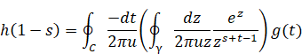
In order to integrate the above equation for the variable z, we deform the above equation as follows.
|
|
(3.23) |
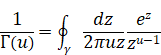
We apply the following formula to the above equation.
(Contour integral formula of the gamma function)
|
|
(3.24) |
Then we obtain get the following equation.
|
|
(3.25) |
|
|
(3.26) |
|
|
(3.27) |
We simplify the above equation by using the following beta function.
|
|
(3.28) |
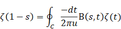
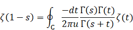
Then, we get the following equation.
(Reflection integral equation)
|
|
(3.29) |
We show the integral path in the following figure. The white circles mean poles.
We show the three-dimensional closed surface S3 in the following figure. The white circles mean poles.
Figure 3.4: The integral path of the reflection formula of the zeta function
4 Conclusion
We obtained the following results in this paper.
- We derived reflection integral equation.
5 Future issues
We show the future issues as follows.
- To study the eigenvalues of integral equation.


