New proof that the sum of natural numbers is -1/12 of the zeta function
Home > Quantum mechanics > Zeta function and Bernoulli numbers
2022/04/16
Published 2014/3/30
K. Sugiyama[1]
Sum of natural numbers of zeta function Z(-1)=1+2+3+… diverges. On the other hand, it is known that analytic continuation of the zeta function ζ(-1)=”1+2+3+…” converges to -1/12. How does the sum of natural numbers approach to -1/12?
In this paper, we prove that the sum of natural numbers decreases and converges to -1/12 after it increases.
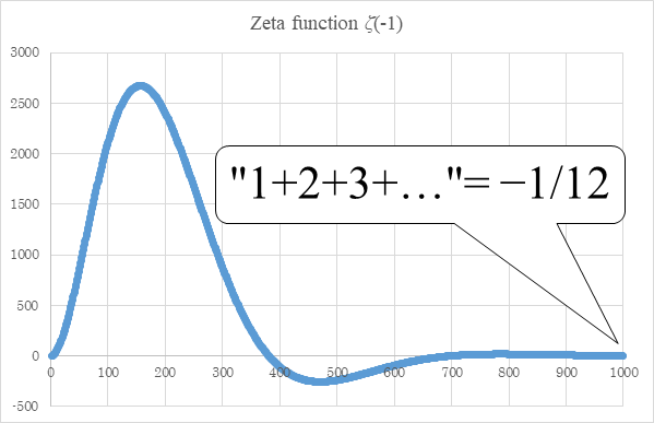
Figure 5.1: Damped oscillation of sum of natural numbers
Abel calculated the sum of the divergent series by the Abel summation method. However, sum of natural numbers diverges even if we use the Abel summation method. In this paper, we calculate the sum of the natural numbers by the damped oscillation Abel summation method.
CONTENTS
1.3 New derivation method of this paper
1.4 Old method by the Abel summation method
2.1 New proof for the summation formula of natural numbers
2.2 Proof of the proposition 1
2.3 Proof of the proposition 2
5.1 Numerical calculation of the oscillating Abel summation method
5.2 General formula of the oscillating Abel summation method
5.3 The mean Abel summation method by residue theorem
5.4 Definitions of the propositions by the (ε, δ)-definition of limit
6.1 Proof of the summation formula of the powers of the natural numbers
6.1.1 Cauchy’s integral formula and mean formula
6.1.2 Laurent series and the pole of the order zero
6.1.3 Introduction of mean harmonic derivative and smooth natural function
6.1.4 Meaning of analytic continuation
6.1.5 The proof of the summation formula of the natural numbers by harmonic derivative
6.1.6 Introduction of mean harmonic overtone derivative and smooth natural overtone function
6.3 Relation with the q-analog
6.4 Relation among zeta function, partition function and harmonic number.
1 Introduction
1.1 Issue
Sum of natural numbers of zeta function Z(-1)=1+2+3+… diverges.
|
|
(1‑1) |
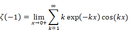
On the other hand, the analytic continuation of the zeta function converges.
|
|
(1‑2) |
How does the sum of natural numbers approach to -1/12? What happens when the normal zeta function Z(s) changes to the analytic continuation of the zeta function ζ(s)?
In order to study the mechanism of the convergence, we try to calculate the sum of natural numbers by Abel summation method.
The normal sum of natural numbers is expressed as follows.
(Normal sum of natural numbers)
|
|
(1.3) |

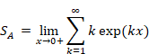
In the Abel summation method, each natural number is multiplied by a damped exponential function to obtain the sum as follows.
(Abel summation method of the sum of natural numbers)
|
|
(1.4) |
By calculating the above equation, the following equation can be obtained.
|
|
(1.5) |
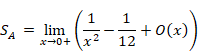
However, unfortunately, the first term 1/x2 diverges. Therefore, the sum of natural numbers diverges even when using the Abel summation method.
It is the purpose of this paper to remove this divergence. In this paper, the sum of natural numbers is calculated by the damped oscillation Abel summation method.
1.2 Research trends so far
Leonhard Euler[2] suggested that the sum of all natural numbers is -1/12 in 1749. Bernhard Riemann[3] showed that the integral representation of the zeta function is -1/12 in 1859. Srinivasa Ramanujan[4] proposed that the sum of all natural numbers is -1/12 by Ramanujan summation method in 1913.
Niels Abel[5] introduced the Abel summation method in order to converge the divergent series in about 1829. J. Satoh[6] constructed q-analogue of zeta-function in 1989. M. Kaneko, N. Kurokawa, and M. Wakayama[7] derived the sum of the double quoted natural numbers by the q-analogue of zeta-function in 2002.
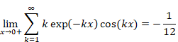
1.3 New derivation method of this paper
We define a new sum of all natural numbers by a new summation method, oscillating Abel summation method (damped oscillation summation method). The method converges the divergent series by multiplying convergence factor, which is damped and oscillating very slowly. The traditional sum diverges for the infinite terms. On the other hand, the new sum is equal to the traditional sum for the finite term. In addition, the sum converges on -1/12 for the infinite term.
(Summation formula of natural numbers)
|
|
(1.6) |
1.4 Old method by the Abel summation method
Niels Abel introduced Abel summation method in about 1829. We consider the following sum of the series.
|
|
(1.7) |

Then we define Abel sum as follows.
(The Abel summation method)
|
|
(1.8) |
|
|
(1.9) |
Abel calculated the sum of the divergent series by the Abel summation method as above stated. However, we cannot calculate the sum of natural numbers by the method. We explain the reason as follows.
We consider the following sum of all natural numbers.
|
|
(1.10) |
Then we define the following function.
|
|
(1.11) |
|
|
(1.12) |
Here, we will use the following formula.
(Formula of the geometric series that has coefficients of natural numbers)
|
|
(1.13) |
We obtain the following equation by the above formula.
|
|
(1.14) |
We calculate the Abel sum as follows.
|
|
(1.15) |
The Abel sum diverges as above stated. Therefore, we cannot calculate the sum of the natural numbers by the Abel sum. In order to examine the mechanism of the divergence, we use the following definitional formula of Bernoulli numbers.
(Definitional formula of Bernoulli numbers)
|
|
(1.16) |
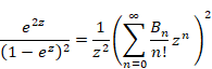
In this paper, Bernoulli numbers Bn is Bernoulli polynomial Bn (1). We will square the both sides of the above formula. In addition, we will divide the both sides by z2. Then we obtain the following equation.
|
|
(1.17) |
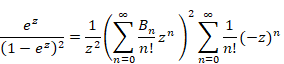
We will multiply the left side of the above formula by e-z. In addition, we will multiply the right side by Maclaurin series of e-z. Then we obtain the following equation.
|
|
(1.18) |
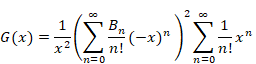
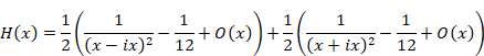
Therefore, we express the function G (x) as follows.
|
|
(1.19) |
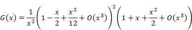
We obtain the following equation by calculating the above formula.
|
|
(1.20) |
|
|
(1.21) |
|
|
(1.22) |
|
|
(1.23) |
|
|
(1.24) |
Here the symbol O (x) is Landau symbols. The symbol means that the error has the order of the variable x. The first term diverges. The first term is called singular term. Therefore, the following the Abel sum diverges.
|
|
(1.25) |
It is the purpose of this paper to remove this divergence.
2 New method
2.1 New proof for the summation formula of natural numbers
We explain the new proof for the summation formula of natural numbers.
We have the following proposition. We will prove the proposition in the next sections.
Proposition 1.
|
|
(2.1) |
We have the following proposition. We will prove the proposition in the next sections, too.
Proposition 2.
|
|
(2.2) |
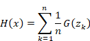
We define the function Sn and Hn (x) as follows.
|
|
(2.3) |
|
|
(2.4) |

Then we define the following symbols.
|
|
(2.5) |
|
|
(2.6) |
|
|
(2.7) |
|
|
(2.8) |
Then we have the following propositions.
|
|
(2.9) |
|
|
(2.10) |
|
|
(2.11) |
The double quotes mean the analytic continuation of the sum of natural numbers.
The traditional sum diverges for the infinite terms. On the other hand, the new “sum” is equal to the traditional sum for the finite term. In addition, the “sum” converges on -1/12 for the infinite term.
2.2 Proof of the proposition 1
Proposition 1.
|
|
(2.12) |
Proof.
We define the function Hn (x) as follows.
|
|
(2.13) |
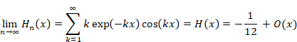
On the other hand, we have the following equation.
|
|
(2.14) |
Therefore, we have the following equation.
|
|
(2.15) |
This completes the proof.
2.3 Proof of the proposition 2
Proposition 2.
|
|
(2.16) |
Proof.
We consider the following sum of all natural numbers.
|
|
(2.17) |
Then we define the following function.
|
|
(2.18) |
|
|
(2.19) |
Here, we use the following formula.
(Euler's formula)
|
|
(2.20) |
We obtain the following formula from the above formula.
|
|
(2.21) |
We obtain the following formula from the above formula by putting θ = k x.
|
|
(2.22) |
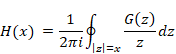
Hence, we express the function H (x) as follows.
|
|
(2.23) |
|
|
(2.24) |
|
|
(2.25) |
|
|
(2.26) |
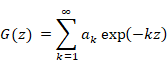
In addition, we define the following function.
|
|
(2.27) |
|
|
(2.28) |
We express the function G (z) from the formula (1.24).
|
|
(2.29) |
Hence, we express the function G (x - ix) as follows.
|
|
(2.30) |
|
|
(2.31) |
Then, we express the function H (x).
|
|
(2.32) |
|
|
(2.33) |
|
|
(2.34) |
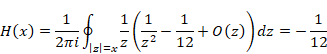
The first term is shown below.
|
|
(2.35) |
On the other hand, the second term is shown below.
|
|
(2.36) |
Therefore, the sum of the first term and the second term vanishes.
|
|
(2.37) |
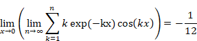
Since the singular term vanished, we have the following equation.
|
|
(2.38) |
We express the function Hn (x) as follows.
|
|
(2.39) |
On the other hand, from the formula (2.38) we have the following equation.
|
|
(2.40) |
Therefore, we have the following equation.
|
|
(2.41) |
This completes the proof.
3 Conclusion
We obtained the following results in this paper.
- We proved that the sum of natural numbers is -1/12 of the value of the zeta function by the new method.
4 Future issues
The future issues are shown below.
- To study the relation between the oscillating Abel summation method and the q-analog.
5 Supplement
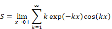
5.1 Numerical calculation of the oscillating Abel summation method
We will calculate the following value numerically.
|
|
(5.1) |
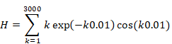
|
|
(5.2) |
This value is very close to the following -1/12.
|
|
(5.3) |
The graph is shown in the Figure 5.1.
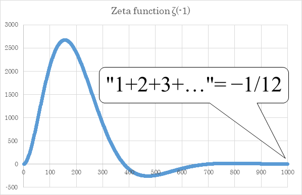
Figure 5.1: Damped oscillation of sum of natural numbers
Here, we will double the attenuation factor as follows. We do not change the vibration period.
|
|
(5.4) |

|
|
(5.5) |
Therefore, the series does not converge if the attenuation factor and the vibration period do not have a special relationship. We will consider the relation in the next section.
5.2 General formula of the oscillating Abel summation method
We consider the following series.
|
|
(5.6) |
Then we define the following function.
|
|
(5.7) |
|
|
(5.8) |
|
|
(5.9) |
In addition, we define the following function.
|
|
(5.10) |
|
|
(5.11) |
We express the function G (z) by using the singular term A (z), and the constant C.
|
|
(5.12) |
Here, we use the following formula.
(Euler's formula)
|
|
(5.13) |
We express the function H (x) as follows by using the above formula.
|
|
(5.14) |
|
|
(5.15) |
|
|
(5.16) |
We obtain the following equation by using the formula (5.12) of the function G (z).
|
|
(5.17) |
We determine the function ![]() by the
following singular equation in order to remove the singular term of the above
equation.
by the
following singular equation in order to remove the singular term of the above
equation.
(Singular equation)
|
|
(5.18) |
The series a k and the
function G (z) and ![]() are shown
below.
are shown
below.
|
Series |
Function |
Function |
|
|
|
|
|
|
|
|
|
|
|
|
|
|
|
|
|
|
|
|
The series and the example of the damped oscillation summation method are shown below.
|
Series |
Example of the damped oscillation summation method |
|
|
|
|
|
|
|
|
|
|
|
|
|
|
|

Therefore, we have the following equations.
|
|
(5‑19) |
|
|
(5‑20) |
|
|
(5‑21) |
|
|
(5‑22) |
We calculate the above equations as follows.
|
|
(5.23) |
|
|
(5.24) |
|
|
(5.25) |
|
|
(5.26) |
General formula of the oscillating Abel summation method is shown below.
|
|
(5.27) |
|
|
(5.28) |
5.3 The mean Abel summation method by residue theorem
We consider the following sum of all natural numbers.
|
|
(5.29) |

Then we define the following function.
|
|
(5.30) |
|
|
(5.31) |
We express the function H (x) as follows.
|
|
(5.32) |
We interpret the above function as a sum of the function G (z1) and G (z2) like the following Figure 5.2.
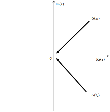
Figure 5.2: The oscillating Abel summation method
In the above Figure 5.2, the two functions G (z1) and G (z2) approach to the origin O at the two angles. This is a special condition. Is it possible to make the condition more general?
Then we consider the case that the many functions G (z) approach to the origin from the all points on the circle of the radius x like the following Figure 5.3.
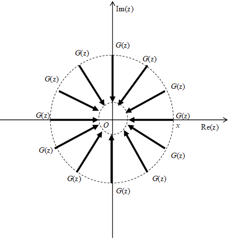
Figure 5.3: The mean Abel summation method
We express the above consideration in the following equations.
|
|
(5.33) |
|
|
(5.34) |
|
|
(5.35) |
|
|
(5.36) |
|
|
(5.37) |
The function H (x) is the contour mean value of the function G (z).
We suppose that the circumference of the circle of the radius x is L. We express the circumference L of the circle as follows.
|
|
(5.38) |
On the other hand, we approximately express the circumference L as follows for sufficiently large n.
|
|
(5.39) |
Therefore, we have the following equation.
|
|
(5.40) |
Then, we express the normalized constant 1/n as follows.
|
|
(5.41) |
|
|
(5.42) |
On the other hand, the direction of -i (zk+1 - zk) is same as the direction of zk as shown in the Figure 5.4.
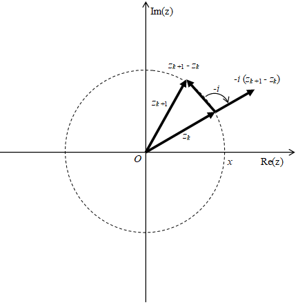
Figure 5.4: General damped oscillation summation method
Therefore, we express 1/n as follows.
|
|
(5.43) |
|
|
(5.44) |
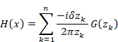
Therefore, we express the function H (x) as follows.
|
|
(5.45) |
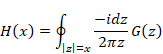
We express the above sum as the following integration.
|
|
(5.46) |
|
|
(5.47) |
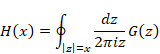
The above result is equal to the residue theorem. We can interpret the residue theorem the mean value theorem of contour integration.
We obtain the following result by the residue theorem.
|
|
(5.48) |
Therefore, we obtain the following new general summation method.
(The mean Abel summation method)
|
|
(5.49) |
|
|
(5.50) |
|
|
(5.51) |
|
|
(5.52) |
This summation method can sum any series by the residue theorem.
5.4 Definitions of the propositions by the (ε, δ)-definition of limit
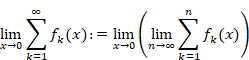
The value of the limit depends on the order of the limit as follows.
|
|
(5.53) |
|
|
(5.54) |
In this paper, we define the order of the limit as follows.
|
|
(5.55) |
|
|
(5.56) |
This order of the limit means the following relation.
|
|
(5.57) |
We confirm the above relation by the (ε, δ)-definition of limit.
In this section, we define the following proposition by the (ε, δ)-definition of limit.
We define the function Sn and Hn (x), and the constant α as follows.
|
|
(5.58) |
|
|
(5.59) |
|
|
(5.60) |

We have the following proposition.
|
|
(5.61) |
We can express the above proposition by (R, N)-definition of the limit as follows.
Given any number R > 0, there exists a natural number N such that for all n satisfying
|
|
(5.62) |
we have the following inequation.
|
|
(5.63) |
We have the following proposition.
Proposition 1.
|
|
(5.64) |
We can express the above proposition by (ε, δ)-definition of the limit as follows.
Given any number x > 0 and any natural number n, there exists a number δ > 0 such that for all x > 0 satisfying
|
|
(5.65) |
we have the following inequation.
|
|
(5.66) |
We can summarize the above definition as follows.
|
|
(5.67) |
We have the following proposition.
Proposition 2.
|
|
(5.68) |
|
|
(5.69) |
We can express the above proposition by (ε, δ)-definition of the limit as follows.
Given any number ε > 0, there exist a natural number N and a number δ > 0 such that for all n satisfying
|
|
(5.70) |
we have the following inequation.
|
|
(5.71) |
We can summarize the above definition as follows.
|
|
(5.72) |
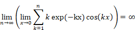
The proposition 1 is the region of 1+2+3+…+n and the proposition 2 is the region -1/12 in the following figure.
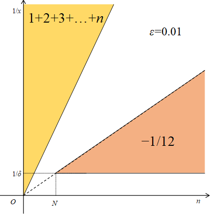
Figure 5.5: (ε, δ)-definition of limit
6 Appendix
6.1 Proof of the summation formula of the powers of the natural numbers
The author found the following formula and proved it in March 2014.
(Summation formula of the natural numbers)
|
|
(6.1) |
N.S found the following formula by generalizing the above formula and published in March 2015.
(Summation formula of the powers of the natural numbers)
|
|
(6.2) |
In this section, we prove the above formula in the following condition.
|
|
(6.3) |
6.1.1 Cauchy’s integral formula and mean formula
When we obtain a new function F (1)(x) by taking a differentiation of a function F(x), we call the function F (1)(x) derivative, and we call the function F(x) generating function.
We express the s order derivative of the function F(q) with respect q as follows.
|
|
(6.4) |
On the other hand, we have the following Cauchy’s integral formula.
(Cauchy’s integral formula)
|
|
(6.5) |
|
|
(6.6) |
The function F(z) of the Cauchy’s integral formula is holomorphic. If the function F(z) is not holomorphic, the integrated function is different from the original function by residue theorem. In this paper, we call the formula with the non-holomorphic function F(z) Cauchy’s mean formula in order to distinguish the Cauchy’s integral formula.
(Cauchy’s mean formula)
|
|
(6.7) |
Here, the counterclockwise contour path goes from the minus infinity to the minus infinity and circles around the point q.
|
|
(6‑8) |
We interpret the function f(q) as the mean value of the values on the contour path C of the function F(z). Therefore, we interpret the Cauchy’s mean formula as the mean value theorem. We interpret the function f (q) is the analytic continuation of the function f (z). We call the analytic continuation of the function the mean function. We use different function name for the function f(q) since the mean function is different from the original function generally.
Cauchy’s differentiation formula is shown below.
(Cauchy’s differentiation formula)
|
|
(6.9) |
|
|
(6.10) |
The function F(z) of the Cauchy’s differentiation formula is holomorphic. In this paper, we call the formula with the non-holomorphic function F(z) Cauchy’s mean differentiation formula in order to distinguish the Cauchy’s differentiation formula.
(Cauchy’s mean differentiation formula)
|
|
(6.11) |
ere, the counterclockwise contour path goes from the minus infinity to the minus infinity and circles around the point q.
|
|
(6‑12) |
We call the function f (s)(q) the mean derivative. We can interpret that the Cauchy’s mean differentiation formula is the formula in order to calculate the mean value of the function and take the derivative of the function. We interpret that the mean derivative is the s order function of the mean value of the generating function.
We express the mean derivative by from derivative by Cauchy’s mean formula.
(Mean derivative)
|
|
(6.13) |
Here, the counterclockwise contour path goes from the minus infinity to the minus infinity and circles around the point q.
|
|
(6‑14) |
We express the generating function by from mean derivative by Laurent series.
(Generating function)
|
|
(6.15) |
The relation between generating function and mean derivative is shown below.

Figure 6.1: Relation between generating function and mean derivative
We can express the above figure as follows.
|
|
(6‑16) |

6.1.2 Laurent series and the pole of the order zero
Generally, the order of the pole is a positive integer n.
(The pole of the order n)
|
|
(6.17) |
|
|
(6.18) |
Though the order of the pole is greater or equal to one generally, we introduce the following the pole of the order zero by using finite positive real number h in this paper.
(The pole of the order zero)
|
|
(6.19) |
|
|
(6.20) |
The pole of the order zero is divergent at z=0. The differentiation of the above pole is shown below.
|
|
(6.21) |
On the other hand, the differentiation of the natural logarithm is shown below.
|
|
(6.22) |
Therefore, we interpret the natural logarithm as the pole of the order zero.
We can derive the constant term C from the coefficient B of the argument of the natural logarithm.
|
|
(6.23) |
Therefore, the new interpretation that we regard the term of the order zero as the pole of the order zero is consistent with the old interpretation that we regard the term of the order zero as the constant term.
We express any function by the new Laurent series with natural logarithm.
(Laurent series with natural logarithm)
|
|
(6.24) |
|
|
(6.25) |
Here, the counterclockwise contour path goes from the minus infinity to the minus infinity and circles around the point O.
|
|
(6‑26) |
We express the function F(z) as follows if the function has the pole of the order zero at most by using the constant A and C.
|
|
(6.27) |
6.1.3 Introduction of mean harmonic derivative and smooth natural function
Harmonic number is shown below.
(Harmonic number)
|
|
(6.28) |

We define the harmonic generating function as follows.
(Harmonic generating function)
|
|
(6.29) |
We use upper letter Η (eta) of Greek letter η (eta) for a symbol of the harmonic generating function.
We obtain the harmonic derivative by computing the s order derivative the harmonic generating function with respect to the variable q.
(Harmonic derivative)
|
|
(6.30) |
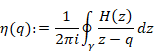
We define the mean harmonic generating function by Cauchy’s mean formula.
(Mean harmonic generating function)
|
|
(6.31) |
Here, the counterclockwise contour path goes from the minus infinity to the minus infinity and circles around the point q.
|
|
(6‑32) |
We define the mean harmonic derivative by Cauchy’s mean formula.
(Mean harmonic derivative)
|
|
(6.33) |
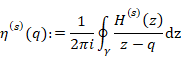
Here, the counterclockwise contour path goes from the minus infinity to the minus infinity and circles around the point q.
|
|
(6‑34) |
We can obtain the mean harmonic derivative by applying Cauchy’s mean differentiation formula to harmonic generating function.
(Mean harmonic derivative)
|
|
(6.35) |
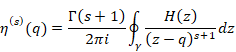
Here, the counterclockwise contour path goes from the minus infinity to the minus infinity and circles around the point q.
|
|
(6‑36) |
The relation between the harmonic generating function and mean harmonic derivative is shown below.
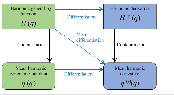
Figure 6.2: Harmonic generating function and mean harmonic derivative
We can express the above figure as follows.
|
|
(6‑37) |

Natural number is shown below.
(Natural number)
|
|
(6.38) |

We define a natural function as follows.
(Natural function)
|
|
(6.39) |
We use upper letter Ν (nue) of Greek letter ν (nue) for a symbol of the natural function.
We obtain the wave natural function by quantizing the natural function.
(Wave natural function)
|
|
(6.40) |
We define the mean wave natural function by Cauchy’s mean formula.
(Mean wave natural function)
|
|
(6.41) |
ere, the counterclockwise contour path goes from the minus infinity to the minus infinity and circles around the point q.
|
|
(6‑42) |
We define the smooth natural function by the classical limit of the above mean wave natural function.
(Smooth natural function)
|
|
(6.43) |
As above stated, we call the operation to quantize a function and calculate the contour mean value of it and take a classical limit smoothing in this paper.
We can obtain smooth natural function by smoothing the natural function as follows.
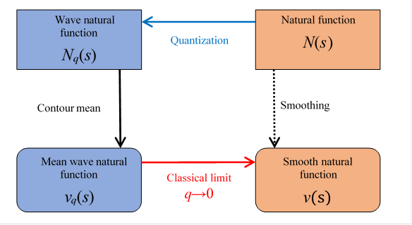
Figure 6.3: We can obtain smooth natural function by smoothing the natural function.
We can express the above figure as follows.
|
|
(6‑44) |

Relation of function in this section is shown below.
|
|
(6‑45) |
6.1.4 Meaning of analytic continuation
What is a meaning of analytic continuation? In this section, we will consider the meaning.
Riemann defined the following zeta function.
(Zeta function)
|
|
(6.46) |

Then, Riemann defined the analytic continuation of zeta function by the following contour integration in 1859.
(Analytic continuation of the zeta function)
|
|
(6.47) |
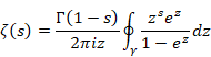
Here, the counterclockwise contour path goes from the minus infinity to the minus infinity and circles around the point O.
|
|
(6‑48) |
Mathematician Weierstrass call the analytic continuation of an analytic function monogenic analytic function in 1842. On the other hand, Mathematician Ahlfors call it global analytic function in 1979. We call it the analytic continuation of the zeta function global zeta function in this paper because I guess the name of the global analytic function is similar to the thought of Riemann.
The global zeta function is different from original zeta function. Then, in order to distinguish original zeta function and global zeta function, we use upper letter Ζ (zeta) of Greek letter ζ (zeta) for a symbol of the original zeta function.
(Zeta function)
|
|
(6.49) |
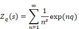
We define the following wave zeta function by multiplying each term of the above summation by exp(nq).
(Wave zeta function)
|
|
(6.50) |
We call the above operation quantization.
We obtain the following mean wave zeta function from the wave zeta function by using Cauchy’s mean formula.
(Mean wave zeta function)
|
|
(6.51) |
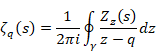
Here, the counterclockwise contour path goes from the minus infinity to the minus infinity and circles around the point q.
|
|
(6‑52) |
We obtain the following global zeta function by taking the classical limit of the above mean wave function.
|
|
(6‑53) |
Analytic continuation means the operation to quantize a function and to take a contour mean value of it and take the classical limit.
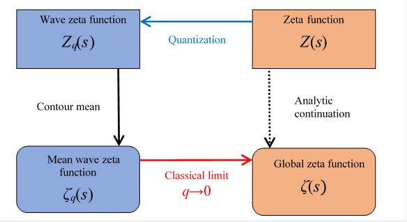
Figure 6.4: Global zeta function
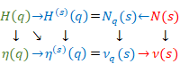
We can express the above figure as follows.
|
|
(6‑54) |

Relation of function in this section is shown below.
|
|
(6.55) |
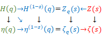
We have the following relation between the smooth natural function and global zeta function.
|
|
(6.56) |
Therefore, the smoothing is same operation as the analytic continuation.
6.1.5 The proof of the summation formula of the natural numbers by harmonic derivative
We choose the following condition.
|
|
(6.57) |
The harmonic generating function is shown below.
(Harmonic generating function)
|
|
(6.58) |
We can modify the above function as follows.
|
|
(6.59) |
We calculate the order of the pole of the harmonic generating function at q=0 by using Landau’s symbol as follows.
|
|
(6.60) |
Since the harmonic generating function has the pole of the order zero at q=0, we express the function as the Laurent series by using the constant A and C.
(Laurent series of the harmonic generating function)
|
|
(6.61) |
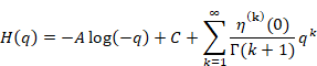
We calculate the second order derivative of the above function.
|
|
(6.62) |
We can prove the summation formula of the natural numbers as follows.
|
|
(6.63) |
|
|
(6.64) |
|
|
(6.65) |
|
|
(6.66) |
(Q.E.D.)
We have the following actual Laurent series of the harmonic generating function.
|
|
(6‑67) |
Therefore, we have the following equations.
|
|
(6‑68) |
|
|
(6‑69) |
|
|
(6‑70) |
|
|
(6‑71) |
|
|
(6‑72) |
|
|
(6‑73) |
|
|
(6‑74) |
6.1.6 Introduction of mean harmonic overtone derivative and smooth natural overtone function
We define the harmonic overtone generating function as follows.
(Harmonic overtone generating function)
|
|
(6.75) |
We obtain the harmonic overtone derivative by computing the s order derivative the harmonic overtone generating function with respect to the variable q.
(Harmonic overtone derivative)
|
|
(6.76) |
We define the mean harmonic overtone derivative by Cauchy’s mean formula.
(Mean harmonic overtone derivative)
|
|
(6.77) |
Relation of the above functions is shown below.
|
|
(6‑78) |
Here, the counterclockwise contour path goes from the minus infinity to the minus infinity and circles around the point q.
|
|
(6‑79) |
We define natural overtone function by taking a classical limit of the mean harmonic overtone derivative.
(Natural overtone function)
|
|
(6.80) |
We can obtain the smooth natural overtone function by applying Cauchy’s mean differentiation formula to harmonic overtone generating function.
(Smooth natural overtone function)
|
|
(6.81) |
Here, the counterclockwise contour path goes from the minus infinity to the minus infinity and circles around the point O.
|
|
(6‑82) |
Relation of function in this section is shown below.
|
|
(6‑83) |
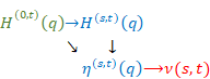
We have the following relation between the smooth natural function and analytic continuation of the zeta function.
|
|
(6.84) |
6.1.7 The proof of the summation formula of the powers of the natural numbers by harmonic overtone derivative
We choose the following condition.
|
|
(6.85) |
Then, we have the following equation for the positive k.
|
|
(6.86) |
In addition, we choose the following condition.
|
|
(6.87) |
Then, we have the following equation for the positive k.
|
|
(6.88) |
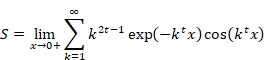
Therefore, we have the following equation by choosing the absolute value of the z is very small.
|
|
(6.89) |
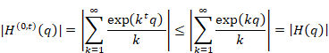
From the above result, we found that the harmonic overtone generating function does not have the pole of higher order than the pole of the harmonic generating function.
We calculate the order of the pole of the harmonic generating function at q=0 by using Landau’s symbol as follows.
|
|
(6.90) |
According to the above result the harmonic generating function has a pole of the order zero at q=0.
Therefore, the harmonic overtone generating function has the pole of the order zero at q=0 at most. Then we express the function as the Laurent series at q=0 by using the function A(t) and C(t).
(Laurent series of the harmonic overtone generating function)
|
|
(6.91) |
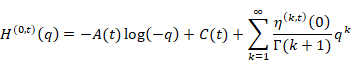
We calculate the second order derivative of the above function.
|
|
(6.92) |
We prove the summation formula of the powers of the natural numbers as follows.
|
|
(6.93) |
|
|
(6.94) |
|
|
(6.95) |
|
|
(6.96) |
(Q.E.D.)
6.1.8 The second proof
In the previous section, we prove the summation formula of the powers of the natural numbers on the following condition.
|
|
(6.97) |
In this section, we prove the formula on the following condition.
|
|
(6.98) |
On the above condition, we have the following formula for the natural number k.
|
|
(6.99) |
Therefore, we have the following formula.
|
|
(6.100) |
In addition, we choose the following condition.
|
|
(6.101) |
Then, we have the following formula for the natural number k and very small z.
|
|
(6.102) |
In the same way, we have the following formula for the natural number k and very small z.
|
|
(6.103) |

Therefore, the absolute value of the following function monotonically decreases.
|
|
(6.104) |
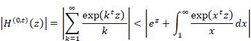
As shown in the following figure, the first term and the integration of the function f(x) from one to infinity is greater than the harmonic overtone generating function.
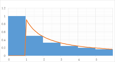
Figure 6.5: Harmonic overtone generating function
Therefore, we have the following formula for very small z.
|
|
(6.105) |
Here, we transform the variable as follows.
|
|
(6.106) |
We take the derivative of the both sides.
|
|
(6.107) |
|
|
(6.108) |
|
|
(6.109) |
|
|
(6.110) |
Therefore, we transform the variable of the integration as follows.
|
|
(6.111) |
Here, we consider the following function.
|
|
(6.112) |
As shown in the following figure, the harmonic generating function is greater than the first term and the integration of the function g(y) from one to infinity.
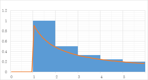
Figure 6.6: Harmonic generating function
Therefore, we have the following formula for very small z.
|
|
(6.113) |
As shown in the previous section, the right side of the following formula has the pole of zero-th at z=0.
|
|
(6.114) |
Therefore, as shown in the previous section, we have the following formula.
|
|
(6.115) |
(Q.E.D.)
6.2 Jacobi’s theta function
Riemann expressed the zeta function by the Jacobi’s theta function.
(The express of the zeta function by the Jacobi’s theta function)
|
|
(6.116) |
|
|
(6.117) |
(Jacobi’s theta function)
|
|
(6.118) |
|
|
(6.119) |
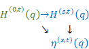
We have the following relation between Jacobi’s theta function and the harmonic overtone generating function.
|
|
(6.120) |
(Harmonic overtone generating function)
|
|
(6.121) |
We obtain the following mean harmonic overtone derivative by using Cauchy’s mean formula.
(Mean harmonic overtone derivative)
|
|
(6.122) |
Here, the counterclockwise contour path goes from the minus infinity to the minus infinity and circles around the point O.
|
|
(6‑123) |
Then, we can obtain the above function by using Cauchy’s mean differentiation formula, too.
|
|
(6.124) |
Here, the counterclockwise contour path goes from the minus infinity to the minus infinity and circles around the point O.
|
|
(6‑125) |
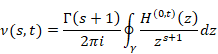
We express the zeta function by the harmonic overtone generating function.
(The express of the zeta function by the harmonic overtone generating function)
|
|
(6.126) |
Here, the counterclockwise contour path goes from the minus infinity to the minus infinity and circles around the point q.
|
|
(6‑127) |
(Harmonic overtone generating function)
|
|
(6‑128) |
6.3 Relation with the q-analog
6.3.1 The q-analog
F. H. Jackson[8] defined the following quantized new natural number, the q-number in 1904.
(The q-number)
|
|
(6.129) |
|
|
(6.130) |
|
|
(6.131) |
We call the quantized mathematical object the q-analog generally. The q-analog of the natural number n is the q-number [n]q. We express the natural number by the classical limit of the q-number.
|
|
(6.132) |
The zeta function is shown below.
(Zeta function)
|
|
(6.133) |

The q-analog of the function is the q-zeta function. The function is shown below.7
(q-zeta function)
|
|
(6.134) |
We express the zeta function by the classical limit of the q-zeta function.
|
|
(6‑135) |
|
|
(6‑136) |
|
|
(6‑137) |
|
|
(6‑138) |

The relation between q-number and the finite harmonic derivative is shown below.
|
|
(6.139) |
|
|
(6.140) |
6.4 Relation among zeta function, partition function and harmonic number.
We define the following finite harmonic derivative.
(Finite harmonic derivative)
|
|
(6.141) |
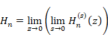
We express the harmonic number by the limit of the finite harmonic derivative.
|
|
(6.142) |
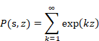
We define the partition function as follows.
(Partition function)
|
|
(6.143) |
We express the partition function by the limit of the finite harmonic derivative.
|
|
(6.144) |
Riemann defined the zeta function.
(Zeta function)
|
|
(6.145) |
|
|
(6.146) |
We express the zeta function by the limit of the h finite harmonic derivative.
|
|
(6.147) |
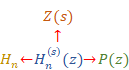
We summarize the above results as follows.
- The harmonic number is the limit of the finite harmonic derivative.
- The partition function is the limit of the finite harmonic derivative.
- The zeta function is the limit of the finite harmonic derivative.
We express these relations in the following figure.
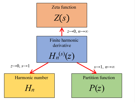
Figure 6.7: Zeta function
We can express the above figure as follows.
|
|
(6‑148) |
7 Acknowledgment
In writing this paper, I thank from my heart to NS who gave valuable advice to me.


