In simple terms, Bell's inequality places an upper limit on the probability that Alice and Bob will meet.
This article explains the meaning of Bell's inequality in an intuitive way, using Venn diagrams.
Bell's inequality can be written as follows:
If this is not the version of Bell's inequality you are familiar with, please see Various Forms of Bell's Inequality below.
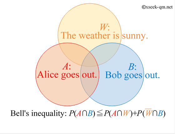
To make the symbols easier to understand, let us replace $W$, $A$, and $B$ with everyday events:
Here, $P(A \cap B)$ is the probability that Alice and Bob both go out. $P(A \cap W)$ is the probability that it is sunny and Alice goes out. $P(\overline{W} \cap B)$ is the probability that it is rainy and Bob goes out, where $\overline{W}$ denotes the case in which it is not sunny.
In everyday language, Bell's inequality says:
The possible cases are as follows:
These cases can be illustrated with the following Venn diagram:
The next figure makes the inequality even clearer.
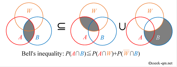
This visual relationship is Bell's inequality. The diagram shows why the overlapping region $A \cap B$ must be contained within the two regions on the right-hand side of the inequality.
Now consider the following situation:
In this situation, Bell's inequality becomes:
With that in mind, consider the following problem.
Under the following conditions, what is the maximum possible probability, in percent, that Alice and Bob will meet?
The answer is 25%. Here is why.
The question asks for the maximum possible probability that Alice and Bob will meet.
We calculate this by separating the cases into sunny days and rainy days. Let us begin with sunny days.
The probability of a sunny day is 50%, and Alice goes out on sunny days with probability 25%. Therefore, the probability $P(A \cap W)$ that it is sunny and Alice goes out is 50% × 25% = 12.5%.
Bob, on the other hand, goes out on sunny days with probability 75%. Thus, the probability $P(B \cap W)$ that it is sunny and Bob goes out is 50% × 75% = 37.5%.
For Alice and Bob to meet on a sunny day, they must both go out. Therefore, the maximum probability that they meet on a sunny day is the smaller of the two probabilities for "sunny and going out," namely $P(A \cap W) = 12.5\%$.
The probability of a rainy day is 50%, and Alice goes out on rainy days with probability 75%. Therefore, the probability $P(\overline{W} \cap A)$ that it is rainy and Alice goes out is 50% × 75% = 37.5%.
Bob, on the other hand, goes out on rainy days with probability 25%. Thus, the probability $P(\overline{W} \cap B)$ that it is rainy and Bob goes out is 50% × 25% = 12.5%.
For Alice and Bob to meet on a rainy day, they must both go out. Therefore, the maximum probability that they meet on a rainy day is the smaller of the two probabilities for "rainy and going out," namely $P(\overline{W} \cap B) = 12.5\%$.
Combining the maximum probability of meeting on a sunny day (12.5%) with the maximum probability of meeting on a rainy day (12.5%), we find that the maximum probability that Alice and Bob meet is 25%.
Therefore, Bell's inequality in this problem is:
Thus, the answer to the question "What is the maximum possible probability that Alice and Bob will meet?" is 25%. As long as the assumptions of the problem are satisfied, no calculation can give a higher probability. This conclusion always holds if the weather can be clearly divided into sunny and rainy cases. Surprisingly, however, in quantum mechanics the left-hand side of this inequality, $P(A \cap B)$, can be 37.5%. The next section explains how this can happen.
Consider the following thought experiment from quantum mechanics:
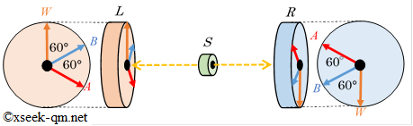
The source $S$ emits one electron toward the left measuring device $L$ and another electron toward the right measuring device $R$. The two electrons form a special pair, called an EPR pair. For example, they may be prepared so that their total spin is zero.
Each measuring device can measure the spin of an electron in a chosen direction. One strange feature of quantum mechanics is that, when measured, the spin of an electron is always found to be either $+1/2$ or $-1/2$ along the chosen direction. If the two electrons have total spin zero and the left device $L$ observes spin $+1/2$ in direction $W$, then a measurement by the right device $R$ in the corresponding direction gives the correlated result. In the notation used here, we focus on the probability of obtaining $+1/2$ on both sides.
From this point on, the explanation becomes a little more mathematical. Suppose the left device $L$ measures the spin of one electron in direction $A$, while the right device $R$ measures the spin of the other electron in direction $B$. Let the angle between directions $A$ and $B$ be $\theta$. According to quantum mechanics, the conditional probability that the right device $R$ observes $+1/2$ in direction $B$, given that the left device $L$ observed $+1/2$ in direction $A$, is given by:
$$ P(B|A) = \frac{ P(A \cap B)}{P(A)}= \cos^2 \left(\frac{\theta}{2} \right) $$Here, $P(B|A)$ is the probability that event $B$ occurs given that event $A$ has occurred. $P(A \cap B)$ is the probability that both events occur at the same time. $P(A)$ is the probability of observing $+1/2$ on the left, which is usually $1/2$ (50%). Here are some examples:
Now let us set up the thought experiment. Take direction $W$ as the reference direction, direction $A$ as $120^\circ$, and direction $B$ as $60^\circ$. Then the angle between $A$ and $B$ is $60^\circ$, while the relevant angles for $A$ and $W$, and for $\overline{W}$ and $B$, are $120^\circ$.
First, calculate the joint probability $P(A \cap B)$. Since the angle difference is $60^\circ$,
$$ P(B|A) = \cos^2 \left(\frac{60^\circ}{2} \right) = \cos^2(30^\circ) = (\sqrt{3}/2)^2 = 3/4 = 75\% $$Since $P(A)=1/2$, the probability $P(A \cap B)$ that both measuring devices obtain spin $+1/2$ is $P(A \cap B) = P(A) \times P(B|A) = (1/2) \times 75\% = 37.5\%$.
$$ P(A \cap B) = 37.5\% $$Next, calculate the joint probability $P(A \cap W)$. Since the angle difference is $120^\circ$,
$$ P(W|A) = \cos^2 \left(\frac{120^\circ}{2} \right) = \cos^2(60^\circ) = (1/2)^2 = 1/4 = 25\% $$Since $P(A)=1/2$, the probability $P(A \cap W)$ that both measuring devices obtain spin $+1/2$ is $P(A \cap W) = P(A) \times P(W|A) = (1/2) \times 25\% = 12.5\%$.
$$ P(A \cap W) = 12.5\% $$Finally, calculate the joint probability $P(\overline{W} \cap B)$. Here, $\overline{W}$ is interpreted as the alternative outcome or opposite direction corresponding to $W$, as used in the diagram. The angle difference between $\overline{W}$ and $B$ is $120^\circ$, so
$$ P(B|\overline{W}) = \cos^2 \left(\frac{120^\circ}{2} \right) = 25\% $$Since $P(\overline{W})=1/2$, the probability is $P(\overline{W} \cap B) = P(\overline{W}) \times P(B|\overline{W}) = (1/2) \times 25\% = 12.5\%$.
$$ P(\overline{W} \cap B) = 12.5\% $$Now let us return to Bell's inequality:
The left-hand side is 37.5%, while the sum on the right-hand side is only 25%. Thus, the predictions of quantum mechanics violate this form of Bell's inequality.
$$ 37.5\% \gt 12.5\% + 12.5\% $$This means that there are strange correlations between the measuring devices $L$ and $R$ that cannot be explained by ordinary classical probability theory. These are called EPR correlations, and they have been confirmed experimentally, for example in Alain Aspect's experiments in 1982.
Where does the mystery of EPR correlations come from? It is thought to arise from the fact that the measurement results $A$ and $B$ cannot be divided into cases based on the unmeasured result $W$ or $\overline{W}$. This is similar to the double-slit experiment: unless we observe which slit the electron passes through, the result cannot be explained simply by dividing the possibilities into "the electron passed through the left slit" and "the electron passed through the right slit."
Let us now consider why Bell's inequality is violated.
In the previous section, I said that the mystery of EPR correlations comes from the fact that the measurement results $A$ and $B$ cannot be classified according to the unmeasured result $W$. Surprisingly, however, it is possible to spatially separate the state corresponding to the unmeasured result $W$. Before explaining this, I will first describe how electron spin is measured.
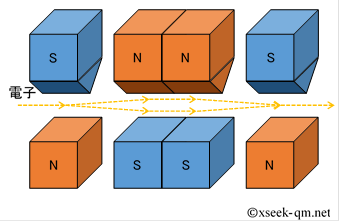
To measure the spin of an electron, we use a Stern-Gerlach apparatus like the one shown below.
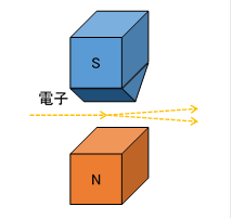
An inhomogeneous magnetic field is created between a pointed south pole and a flat north pole. The magnetic field becomes stronger closer to the south pole. When an electron beam passes through this inhomogeneous magnetic field, the beam splits into two paths depending on the direction of the electron's spin. This makes it possible to determine the spin direction, up or down, relative to the direction of the measuring magnetic field. Regardless of the original spin direction, the electron is always found in one of the two paths relative to the direction being measured.
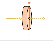
By combining Stern-Gerlach apparatuses, we can construct the following device.
In this device, the electron beam first splits and then recombines. For the explanation below, I will represent this device using the following simplified diagram.
What happens if we place a wall $C$ in the middle of the device?
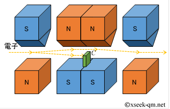
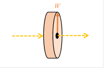
Since the lower path is blocked, the path taken by the electron becomes definite: in this case, it must have taken the upper path. For the explanation below, I will represent the device with one path blocked using the following simplified diagram.
Using these devices, let us consider the following thought experiment.
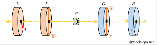
One electron of the EPR pair first passes through device $F$, which separates and recombines the beam according to direction $W$, and is then sent to device $L$, which measures in direction $A$. The other electron similarly passes through device $G$, which separates and recombines the beam according to direction $W$, and is then sent to device $R$, which measures in direction $B$. In devices $F$ and $G$, the electron beam is temporarily separated into the paths $W$ and $\overline{W}$ according to the spin direction and then recombined. Even so, EPR correlations can still appear between the results obtained by devices $L$ and $R$, and these correlations can violate Bell's inequality.
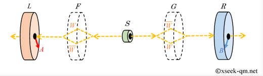
This is a very mysterious result. While the electron beam is separated into the two paths $W$ and $\overline{W}$, it seems possible, at least in principle, to determine which path the electron is on. If the cases could really be divided according to the path, that is, according to the result of a measurement in direction $W$, then Bell's inequality should hold. Why, then, is Bell's inequality violated?
If we actually perform a measurement that determines the path while the electron beam is separated into the paths $W$ and $\overline{W}$, for example by blocking one path, then Bell's inequality holds. However, if the two paths are recombined without determining which path the electron took, the two possibilities interfere with each other. As a result, correlations appear that violate Bell's inequality. These correlations show that the two distant electrons still form a single combined quantum state, that is, an entangled state. The reason for the violation of Bell's inequality can therefore be summarized as follows:
In fact, several different inequalities are commonly referred to as Bell's inequality. I will briefly introduce a few of them here.
The Irish physicist John Bell proposed the first version in 1964. It was written in terms of a correlation function $C$.
Here, $C(A,B)$ represents the strength, or expectation value, of the correlation between measurement results in directions $A$ and $B$. However, the meaning of this inequality is not easy to grasp intuitively. Later, in 1969, Clauser, Horne, Shimony, and Holt proposed the following inequality, now known as the CHSH inequality, in a form better suited to experimental tests.
This inequality is also written in terms of correlation functions. Around 1970, the Hungarian physicist Eugene Wigner reformulated Bell's inequality using probabilities. A similar form was also discussed by Bernard d'Espagnat.
In his well-known textbook Modern Quantum Mechanics, first published in 1994, the physicist J. J. Sakurai introduced the probability-based form above as Bell's inequality. Here, $P(A+;B+)$ represents the joint probability that, in the EPR experiment below, the left measuring device $L$ observes spin $+1/2$ in direction $A$ ($A+$), and the right measuring device $R$ observes spin $+1/2$ in direction $B$ ($B+$).
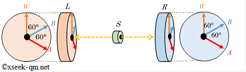
Bell's original inequality from 1964 and the CHSH inequality from 1969 are written in terms of the strength of correlations, or expectation values. By contrast, the Wigner-d'Espagnat inequality from around 1970 is written in terms of probabilities. This makes the meaning of the inequality easier to understand, although it is still not completely obvious at first glance. One reason is that the directions $A$, $B$, and $W$ for the left measuring device $L$ and the corresponding directions for the right measuring device $R$ are treated in the same way. Because the two sides are inversely correlated, it becomes easier to understand the inequality if the directions for the right measuring device $R$ are rotated by 180 degrees, as shown below.
Based on this EPR experiment, the meaning of Bell's inequality becomes more intuitive if it is written in set notation:
$$ P(A \cap B) \leqq P(A \cap W)+P(\overline{W} \cap B) $$This is the form of Bell's inequality used throughout this article. It can be represented by the following Venn diagram.
The Venn diagram makes the meaning of Bell's inequality much clearer. In fact, the French physicist Bernard d'Espagnat also explained Bell's inequality using a Venn diagram in 1979 (reference link).
Bell's inequality holds if the weather can be divided into sunny and rainy cases. In physics, this corresponds to the assumptions behind local realism. In quantum mechanics, however, unless the relevant property is actually measured, it cannot always be divided into such definite cases.
If Alice meets Bob and someone asks what the weather was like that day, what answer would they give? Strangely enough, in the quantum world, unless the weather is measured, the weather condition remains indeterminate.
© 2002-2018 xseek-qm.net
広告


