Derivation of the Born rule from many-worlds interpretation and probability theory

 

Home  >  Quantum mechanics  >  Derivation of Born rule of quantum mechanics

 

2019/02/20

Published 2012/09/26

K. Sugiyama^[1]

 

Born rule is a rule that a probability we observe a small particle like an electron is proportional to the square of the absolute value of the wave function. In this paper, we try to derive the Born rule from the many-worlds interpretation.

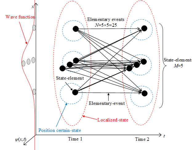
Figure 3-6: Derivation of Born rule by the network structure of the path integral

 

Many researchers have tried to derive the Born rule (also called Born’s rule, Born's law, or probability interpretation) from many-worlds interpretation (MWI). However, nobody succeeded. Thus, the derivation of Born rule had become an important issue for MWI. We try to derive Born rule by introducing an elementary-event (also called an atomic event or simple event) of probability theory to the quantum theory as a new method.

 

The absolute value of a wave function is regarded as a surface area of a manifold. A position on the surface of the manifold is regarded as an elementary-position. A particle existing at the elementary-position is regarded as a state-element. The state that the state-element existing at the elementary-position is regarded as an elementary-state. A transition from one elementary-state to the other elementary-state is regarded as an elementary-event.

 

A probability is proportional to the number of elementary-events, and the number of elementary-events is the square of the number of elementary-states. The number of elementary-states is proportional to the surface area of the manifold, and the surface area of the manifold is an absolute value of a wave function. Therefore, the probability is proportional to a square of an absolute value of a wave function.

 

CONTENTS

1       Introduction. 1

1.1       Subject 1

1.2       The importance of the subject 1

1.3       Past derivation method. 1

1.4       New derivation method of this paper 1

2       Traditional method of deriving and the problem.. 1

2.1       The Born rule. 1

2.2       Everett's many-worlds interpretation. 1

2.2.1    The basis problem of many-worlds interpretation. 1

2.2.2    The probability problem of many-worlds interpretation. 1

3       A new method of deriving. 1

3.1       Elementary-event of many-worlds interpretation. 1

3.2       Elementary-states of many-worlds interpretation. 1

3.3       Introduction of a elementary-state to the quantum theory. 1

3.4       Application of path integral to the field. 1

3.5       Introduction of elementary-event to the quantum theory. 1

3.6       Derivation of Born rule. 1

4       Conclusion. 1

5       Supplement 1

5.1       Supplement of the many-particle wave function. 1

5.2       Supplement of the method of deriving Born rule. 1

5.3       Supplement of basis problem in many-worlds interpretation. 1

5.4       Interpretation of time in many-worlds interpretation. 1

5.5       Supplement of long distance transition. 1

5.6       Supplement of observation. 1

6       Future Issues. 1

7       Consideration of the future issues. 1

7.1       Consideration of principles. 1

7.1.1    Hierarchical principle. 1

7.1.2    Event principle. 1

7.2       Consideration of formulation for the quantum field theory. 1

8       Appendix: Review of existing ideas. 1

8.1       Universal Wave function of Wheeler and DeWitt 1

8.2       Barbour's many-particle wave function of the universe. 1

8.3       Laplace's Probability Theory. 1

8.4       Penrose's spin networks. 1

8.5       Feynman's path integral 1

8.6       Dirac's quantum field theory. 1

8.7       Kaluza-Klein theory. 1

9       Appendix: Review of existing ideas (part 2) 1

9.1       Euler’s formula. 1

9.2       Cauchy-Riemann equation. 1

9.3       Hamilton’s Quaternion. 1

9.4       Cauchy-Riemann-Fueter equation. 1

9.5       Cartan's differential form.. 1

10     Appendix: Hierarchical universe. 1

10.1     Universe of Two-dimensional space-time. 1

10.1.1      Closed path of Two-dimensional space-time. 1

10.1.2      Introduction of the absolute value of wave function. 1

10.1.3      Introduction of the phase of wave function. 1

10.1.4      Hierarchical universe. 1

10.1.5      Equations. 1

10.2     Universe of four-dimensional space-time. 1

10.2.1      Closed path of four-dimensional space-time. 1

10.2.2      Introduction of the absolute value of wave function. 1

10.2.3      Introduction of the phase of wave function. 1

10.2.4      Hierarchical universe. 1

10.2.5      Equations. 1

10.3     Normal space. 1

10.4     Wave space-time. 1

11     Appendix: Terms. 1

11.1     Definition of Terms. 1

11.2     Arrangement of Terms. 1

12     Acknowledgment 1

13     References. 1

 

1       Introduction

1.1      Subject

According to Born rule, an observed probability of a particle is proportional to the square of the absolute value of the wave function. It is the subject of this paper to derive Born rule by counting the number of the events.

 

1.2      The importance of the subject

Wave function collapse and Born rule are the principle of the quantum mechanics. We can eliminate the wave function collapse from the quantum mechanics by many-worlds interpretation (MWI), but we cannot eliminate Born rule. For this reason, many researchers have tried to derive Born rule from MWI. However, it has not resulted in the success. Therefore, it has become an important subject to derive Born rule.

 

1.3      Past derivation method

Hugh Everett III^[2] claimed that he derived Born rule from many-worlds interpretation (MWI) in 1957. After that, many researchers claimed that they derived Born rule from the method that is different from the method of Everett. James Hartle^[3] claimed in 1968, Bryce DeWitt^[4] claimed in 1970 and Neil Graham^[5] claimed in 1973 that they derived Born rule. However, Adrian Kent pointed out that their method of deriving Born rule was insufficient^[6] in 1990. David Deutsch^[7] tried to derive Born rule.in 1999. Sumio Wada^[8] also tried it in 2007. However, many researchers do not agree on the methods of deriving Born rule.

 

1.4      New derivation method of this paper

In probability theory, we had explained the probability by the concept of an elementary-event (also called an atomic event or simple event). Therefore, we might be able to explain the probability of the quantum theory by the same concept. We try to derive the probability of the quantum theory by introducing a concept of an elementary-event to the quantum theory as the new method of this paper.

 

2       Traditional method of deriving and the problem

2.1      The Born rule

Max Born^[9] proposed the Born rule in 1926. It is also called Born’s  rule, the Born law, the Born's law, or the probability interpretation. Born rule is a principle of quantum mechanics. We express the state of the particle by the wave function ψ (x) in quantum mechanics. We show an example of the wave function in the following figure.

 

Figure 2-1: An example of a wave function

 

The observed probability of a particle is proportional to the square of the absolute value of the wave function. We express the observed probability P (x) of a particle at the position x as follows.

 

 

According to the Copenhagen interpretation that is a general interpretation of quantum mechanics, we cannot describe the state of the particle before the observation because the wave function does not exist physically. However, the wave function might exist physically. One of the interpretations based on the existence of a wave function is many-worlds interpretation.

 

2.2      Everett's many-worlds interpretation

Everett proposed many-worlds interpretation (MWI) in order to deal with the universal wave function. He tried to derive Born rule from the measure.

 

For example, we consider the Stern-Gerlach experiment. We can express the state of spin in any direction by superposition of spin-up state along z-axis and spin-down state along z-axis. Therefore, we express the state vector of the spin of an electron by the eigenstate vector of the spin along the z-axis as follows.

The coefficients a and a_k are complex number. Here, we have normalized |ψ>, |z+> and, |z−> as follows.

 

In order to derive the probability, Everett introduced a new concept, measure. He expressed the measure by a positive function m(a). He requested the following equation for the measure.

 

He adduced a probability conservation law to justify the request. We write the function m(a) satisfying the above equation by using a positive constant c as follows.

Andrew Gleason^[10] generally proved the above equation in 1957. His proof is called the Gleason's theorem. Everett considered the infinite time measurement, and concluded that the measure behaves like the probability. However, MWI of Everett has a basis problem and a probability problem. I will explain them in the following sections.

 

2.2.1        The basis problem of many-worlds interpretation

If we define the measure by using a particular basis, we need to show how to select a particular basis. However, Everett did not show how to select a particular basis in his paper.

 

We can express the wave function of an electron by the basis of the spin eigenstate along z-axis as follows.

We can express the measure of the spin eigenstate along z-axis as follows.

On the other hand, we can also express the wave function of an electron by the basis of the spin eigenstate along x-axis as follows.

We can express the measure of the spin eigenstate along x-axis as follows.

 

If the measure of Everett is a quantity that exists physically, it should not change by choice of a basis of eigenstate, because a quantity that exists physically does not depend on the method to observe it. Therefore, we need a method to choose a specific basis. However, Everett did not show the method.

 

2.2.2        The probability problem of many-worlds interpretation

Everett tried to derive Born rule from the measure theory. Then, Everett did not give the physical meaning to the measure. However, to request the conservation law of the probability for the equation of the measure is equivalent to defining the measure as the probability. Therefore, it is circular reasoning to show that measure acts like a probability for infinite time measurement.

 

If the number of worlds is proportional to the measure, it is necessary to clarify the mechanism that the number of worlds is proportional to the measure. If the number of worlds is not proportional to the measure, it is necessary to explain how the probability of occurrence of a world is proportional to the measure.

 

3       A new method of deriving

3.1      Elementary-event of many-worlds interpretation

We introduce elementary-events to quantum mechanics by embracing the many-worlds interpretation (MWI) in this paper.

 

If we interpret an event of quantum theory as a set of elementary-events, we can derive the probability of an event by counting the number of elementary-events that belong to the event. If the event R or event B occurs in some observations, a history branches to the history that event R occurs and the other history that event B occurs in the many-worlds interpretation.

 

For example, if the number of elementary-events of the event R is three, and the number of elementary-events of the event B is two, the probability of occurrence of the event R is 3/5.

 

Figure 3-1: A history is a set of elementary histories in many-worlds interpretation

 

The concrete implementation method of elementary-events is described in the following sections.

 

3.2      Elementary-states of many-worlds interpretation

In the wave function of a many-particle system in configuration space (many-particle wave function), we call the state (position eigenstate) that positions of all particles are decided a position certain-state, or certain-state.

 

In the actual experiment, a particle spreads in the narrow range. Therefore, actual state diffuses in the narrow range in configuration space. We can regard the state as the set of the certain-states. We call the state a localized-state.

 

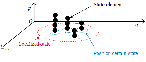
Figure 3-2: Elementary-states in configuration space

 

The absolute value of a wave function is regarded as a surface area of a manifold. A position on the surface of the manifold is regarded as an elementary-position. A particle existing at the elementary-position is regarded as a state-element. The state that the state-element existing at the elementary-position is regarded as an elementary-state.

 

In the discussion of this paper, there is no difference between the discussion using the many-particle wave function and the discussion using the wave function of one particle. Therefore, in the discussion of this paper, we do not use the many-particle wave function but the wave function of one particle.

 

3.3      Introduction of a elementary-state to the quantum theory

We express the wave function ψ(x) by Dirac delta function as follows.

 

 

We interpret the state ψ(x')δ(x − x') as the state that the position x of the particle is fixed at the position x', "Certain-state." The state δ(x − x') is regarded as an elementary-state. K. Sugiyama^[11] introduced the elementary-state in 1999.

 

We divided the virtual high-dimensional Euclidean space by using "elementary domain" and we suppose that lattice points are elementary-states. The certain-state is 1-sphere or 3-sphere and the lattice points on the sphere are elementary-states of the certain-state.

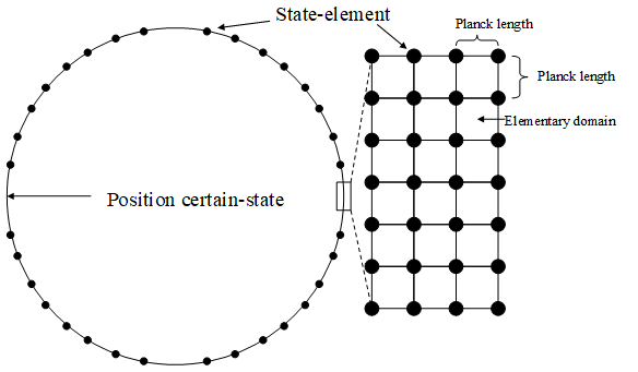
Figure 3-3: Elementary-states of many-worlds interpretation

 

 Since the surface area S of the manifold is the absolute value |ψ (y, t)| of the wave function, we describe the number M (y, t) of the elementary-states by using Planck length  as follows.

 

 

3.4      Application of path integral to the field

In quantum field theory, we apply path-integral to field. On the other hand, the state-elements construct the field. Therefore, we apply to the state-elements.

 

We introduce a new wave function Ψ that has an argument of a wave function ψ.

 

There is a network structure of the path integral for the position x that is "positional physical quantity." (See section 8.5.)  Therefore, we apply a network structure of the path integral for the field ψ that is "positional physical quantity" like the following figure.

 

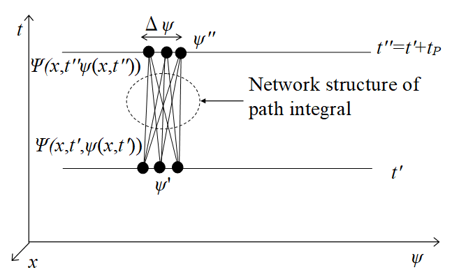
Figure 3-4: Application of network structure of path integral to field itself

 

In the above figure, we apply the "network structure of the path integral" to the region that is smaller than Δψ.

 

3.5      Introduction of elementary-event to the quantum theory

We introduce a new concept, an elementary-event to the quantum theory in this paper.

 

We express an event as a transition from one state to the other state in quantum theory. Therefore, we express an elementary-event as a transition from one elementary-state to the other elementary-state.

 

If the arrow from the point A to the point B exists, the arrow from the point B to the point A also exists conversely. If the number of points is M, the number of arrows becomes M ². In other words, if the number of elementary-states is M, the number of elementary-events becomes M ².

 

Though there is no clear evidence of the existence of an elementary-event, we deduce it by the following reasons.

 

 

 

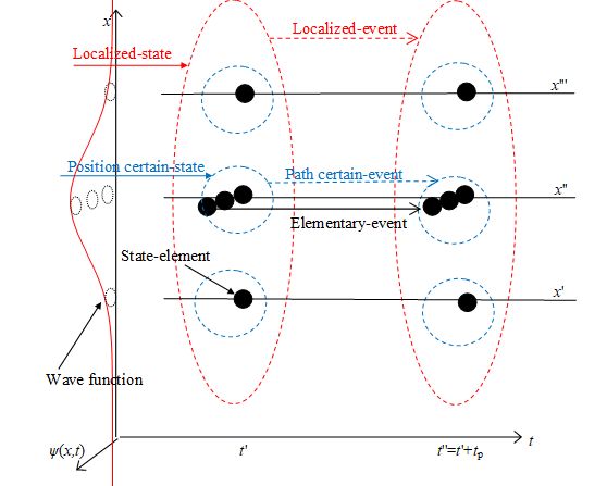
Figure 3-5: Elementary-states and elementary-events of many-worlds interpretation

 

We assume that the elementary-event of this paper have the same properties of elementary-events (also called an atomic event or simple event) of probability theory. In other words, the probability of occurrence of an event is proportional to the number of elementary-events those are included in the event.

 

In addition, we define the event that is a transition from any Certain-state to any Certain-state "Certain event." The Certain event is a set of elementary-events.

 

Actual states are localized by the uncertainty principle. We call the states localized-states. We call the event from any localized-state to any localized-state a "Localized-event."

 

If we apply the path integral to the discrete space-time, the long distance transition from Certain-state occurs. However, "long distance transition" is suppressed due to the localized-states. It means that the number of elementary-events of Localized-event that is Long distance transition is very rare.

 

The existence of elementary-states and elementary-events suggests that an existence probability and a probability of occurrence are different concepts. If the number of elementary-states of a state is m, the state existence probability is proportional to m. If the number of elementary-events of an event is n, the event's existence probability is proportional to n.

 

3.6      Derivation of Born rule

This section describes how to derive this probability.

 

We express the observation probability P(x, t) of the particle by the wave function ψ(x, t) as follows.

 

 

On the other hand, we express the probability P based on the Laplace's calculation method of the probability as follows.

 

 

Here N_a is the number of all elementary-events and N is the number of elementary-events those are expected. If N_a is sufficiently larger than N, the probability P is proportional to N.

 

 

Actual state is localized-state. We apply the "network structure of path integral" to the localized-state. Since "long distance transition" does not occur for localized-state, the length of transition is small after a minimum time t_P.

 

The number M (x', t') of elementary-events of the localized-state ψ (x', t') Δx is proportional to the surface area of the manifold. We apply the "network structure of path integral" to the position on the surface area of the manifold.

 

 Since the manifold after the minimum time almost same as the original manifold, we approximate it by the same manifold. We express the number M (x, t) of elementary-states on the surface area of the manifold as follows.

 

Therefore, the number of the elementary-states is proportional to the absolute value of the wave function if the Δx is almost constant.

 

According to the uncertainty principle, the deviation Δp of momentum is almost constant if Δx is almost constant. Therefore, the number M of the elementary-states approximately does not change for Planck time t_P.

 

The number N of elementary-events is the number of transitions from all elementary-states at time 1 to all elementary-states at time 2 after Planck time t_P. Therefore, the number N of elementary-events is the square of the number M of elementary-states.

 

We express those elementary-events in the following figure.

 

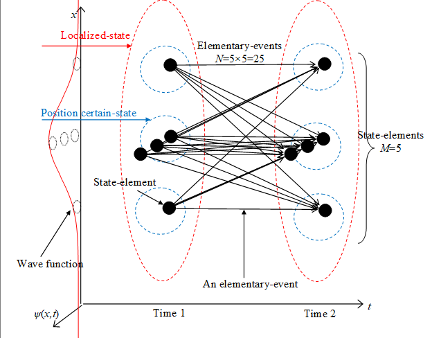
Figure 3-6: Derivation of Born rule by the network structure of the path integral

 

The probability P is proportional to the number of the elementary-events N.

On the other hand, the number N of the elementary-events is equal to the square of the number M of elementary-states.

The number M of elementary-events is proportional to the absolute value of the wave function.

Therefore, the probability P is proportional to the square of the absolute value of the wave function.

We derived the Born rule by the above method.

 

4       Conclusion

We explained the method to derive Born rule from many-worlds interpretation and probability theory.

 

Probability is proportional to the number of elementary-events. The number of elementary-events is the square of the number of elementary-states because we apply the "network structure of path integral" to the elementary-state. The number of elementary-states is proportional to the absolute value of the wave function. Therefore, the probability is proportional to the absolute value of the wave function.

 

 

5       Supplement

5.1      Supplement of the many-particle wave function

We call an elementary-state, a certain-state and a localized-state for the universe "world-element," "certain-world" and "localized-world" respectively.

 

In addition, we call an elementary-event, a certain-event and a localized-event for the universe "elementary-history", "certain history" and "localized-history" respectively.

 

Figure 5-1: Elementary-history and world-element of many-worlds interpretation

 

We interpret one point of the configuration space of the many-particle wave function as the state that the positions of all particles are determined. The state is "certain-world."

 

In the view of classical mechanics, the point is our world. In the view of the quantum mechanics, localized-world is our world.

 

I guess that the absolute value of the many-particle wave function of the universe is most nearly zero in the almost area. The domain that the absolute value is large is localized like a network structure.

 

5.2      Supplement of the method of deriving Born rule

The simplest way to derive Born rule from many-worlds interpretation (MWI) is that we connect the number of worlds to the probability.

 

If the probability of occurrence of event A is higher than the probability of occurrence of event B, we deduce that the number of worlds those event A occurred is greater than the number of worlds those event B occurred.

 

For example, we suppose that we make the 100 planets those are exactly same as Earth. If the event A occurred on 80 planets and the event B occurred on 20 planets, then we interpret that the probability of the occurrence of the event A is 80%.

 

However, it is not clear how to count the world. Therefore, we count the number of world-elements of the localized-world that event A occurred.

 

We express the number M of world-elements of the localized-world by the wave function ψ that event A occurred as follows.

 

Δx is the position deviation, and n is the number of all particles. The number of world-elements is proportional to the absolute value of the wave function.

On the other hand, the probability is proportional to the square of the absolute value of the wave function. Therefore, we cannot explain the probability by using the number of the world-elements.

 

To solve this problem, we explain the probability by using the number of histories. We express the number N of elementary histories of the localized-history that event A occurred as follows.

 

 

The probability is proportional to the number of elementary histories.

The number of histories is the square of the number of world-elements.

On the other hand, the number of the world-elements is proportional to the absolute values of the wave function.

Therefore, the probability is proportional to the square of the absolute value of the wave function.

 

5.3      Supplement of basis problem in many-worlds interpretation

In many-worlds interpretation, the absence of a particular basis of the wave function is a problem.

 

For example, we consider the Stern-Gerlach experiment of the spin of electrons. In this experiment, we measure the spin by using a magnetic field gradient. Since the basis of the spin is determined by the direction of the gradient magnetic field, there is no particular basis for the spin.

 

In this paper, we chose position as the particular basis. We could also choose the momentum as the particular basis, but we did not do so, because we express the basis of the momentum by using a set of elementary-states those the positions are basis.

 

For spin, there is no way to select a particular basis. Therefore, we encounter the problem that the measure changes by choosing the basis of spin. The cause of the problem is in an interpretation that one elementary state construct a state that has a particle of spin-up.

 

I showed that we can derive the spin from the rotation of 3-sphere in the following paper.

・Derivation of two-valuedness and angular momentum of spin-1/2 from rotation of 3-sphere [2013/5]

https://xseek-qm.net/Spin_e.htm

 

If the spin is rotation 3-sphere, we can interpret that many elementary states construct a state that has a particle of spin-up. Choosing the basis of spin is equivalent to changing the observation axis of the 3-sphere. The observation decide a set of elementary states those belong to spin-up state and a set of elementary states those belong to spin-down state. Therefore, we can solve the basis problem of MWI by the rotation of 3-sphere.

 

5.4      Interpretation of time in many-worlds interpretation

The position of all particles is different for a point in the configuration space of many-particle wave function. Therefore, we define the time for a point in the configuration space. Since a point corresponds to a certain-world, we interpret the time as a parameter to classify the certain-worlds.

 

A certain-world transits the minimum length continuously in the configuration space. I guess that we feel the transition as a time.

 

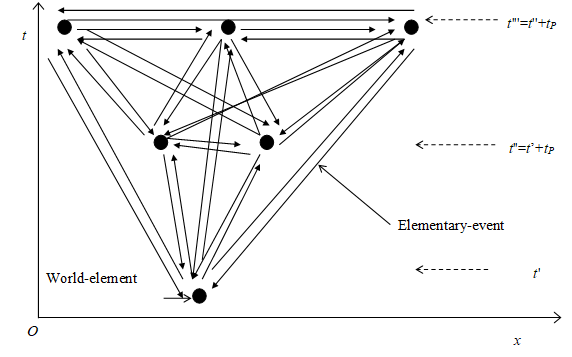
Figure 5-2: Many-worlds interpretation and arrow of time

 

If a transition of a direction exists, the transition of the opposite direction also exists. However, since there are many "world-elements" of future more overwhelmingly than the number of world-elements of past, we feel that our world-element always transits to world-element of the future. In this way, many-worlds interpretation explains the arrow of time by.

 

5.5      Supplement of long distance transition

In this paper, we have been thinking about one particle is localized in one place. Here we consider the wave function of one particle that was localized in one place at a time. We suppose that the wave function was separated and localized in two places. We call the state "many localized-states." In this case, what would happen?

 

Elementary-event exists between any two elementary-states. The world does not become disorder because long distance transition is suppressed due to the "localized-state." We determine the number of elementary-events between two localized-states only by the number of elementary-states of the two localized-states.

 

Therefore, if there are "many localized-states," the transition between two localized-states will occur.

 

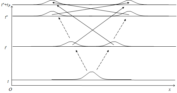
Figure 5-3: Long distance transition between localized-states

 

I call the phenomenon "localized long distance transition" or "localized shift."

 

Then, will localized shift between localized-states those have different time occur?

 

In this case, since the elementary-event exists between any two elementary-states, the localized shift occurs, too.

 

I do not deduce that the localized teleport send information, because we cannot send any information by using EPR correlation.

 

5.6      Supplement of observation

Observation is an operation to transform uncertain information entropy Q to certain information entropy H as follows.

 

We define certain information entropy H for the observed information as follows.

(Certain information entropy)

 

We define the uncertain information entropy Q for the unobserved wave function ψ (x) as follows.

(Uncertain information entropy)

 

We define uncertain information entropy Q for the unobserved angular momentum of the k-th particle as follows.

(Uncertain information entropy)

 

We define the general information entropy G.

(General information entropy)

This general information entropy conserves.

 

(Law of general information entropy conservation)

 

Certain information entropy always increases by a thermodynamics second law.

(Law of entropy increase)

 

However, certain information entropy has the following upper limit because of uncertainty principle.

(Upper limit of certain information entropy)

All the particle’s angular momentums of y-direction and z-direction become uncertain, when all the particle’s angular momentums of x-direction are observed.

 

Certain information entropy increases when the wave function collapses.

Uncertain information entropy increases when the wave function diffuses (anti-collapses).

 

If we make a status uncertain status, uncertain information entropy increases.

 

6       Future Issues

Future issues are shown as follows.

 

(1)   Consideration of the principle

(2)   Formulation for the quantum field theory

(3)   Consideration of the discrete space

(4)   Formulation for the relativistic mechanics

(5)   Formulation for the gravity theory

 

We consider some of these issues in the following chapters.

 

7       Consideration of the future issues

7.1      Consideration of principles

We consider the hierarchical principle and the event principle.

 

7.1.1        Hierarchical principle

I propose the following hierarchical principle.

 

(1)   Wave functions are quaternionic functions.

(2)   The direct product of the closed path of a particle and the wave function is the other universe.

(3)   Wave functions in the other universe are also quaternionic functions.

 

We call the theory based on the hierarchy principle the hierarchy theory.

 

7.1.2        Event principle

I propose the following event principle.

 

(1)   An elementary-event is the transition from an elementary-state to the other elementary-state.

(2)   Event probability of an event is proportional to the number of elementary-events those the event includes.

 

We call the theory based on the event principle the event theory.

 

7.2      Consideration of formulation for the quantum field theory

A certain-state has a phase and an absolute value of the wave function. Therefore, it is possible to use “suppression of long distance transition due to localized-states” for the certain-state. On the other hand, an elementary-state does not have a phase and an absolute value of the wave function. Therefore, it is impossible to use “suppression of long distance transition due to localized-states” for the elementary-state. In order to solve the problem, we consider the quantum field theory.

 

In the quantum mechanics, the position and the momentum of a particle have a commutation relation. It means that the position of the particle is distributed. On the other hand, in the quantum field theory the amplitude and the general momentum of the wave function have a commutation relation. It means that the amplitude of the wave function is distributed.

 

Then I propose the following new function.

We call the function the second wave function because we get the wave function by the second quantization of the field. The second wave function exists in the second universe. The elementary-state of the first universe is the certain-state of the second universe. Therefore, it is possible to use “suppression of long distance transition due to localized-states” for the elementary-state.

 

8       Appendix: Review of existing ideas

8.1      Universal Wave function of Wheeler and DeWitt

John Wheeler and Bryce DeWitt^[12] proposed the universal wave function in 1967. We have the wave function by the Hamiltonian operator H and the ket vector |ψ> as follows.

 

 

This ket vector |ψ> is not a normal function but a functional.

 

A functional is mathematically almost equivalent to a function of many variables. Since the discussion based on the functional is difficult, we use a function of many variables for discussion in this paper. The following sections describe the many-particle wave function, which is a function of many variables.

 

8.2      Barbour's many-particle wave function of the universe

Julian Barbour^[13] expressed the universe by using the many-particle wave function in his book The End of Time in 1999.

 

We suppose that the number of the particles in the universe is n, and the k-th particle's position is r_k = (x_k, y_k, z_k). Then we express the many-particle wave function ψ as follows.

 

 

The many dimensional space expressing the positions of all the particles is called configuration space.

 

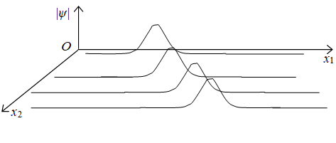
Figure 8-1: Many-particle wave function

 

The configuration space expresses all the possible worlds those exist physically in the past, the present, and the future, because a point in the configuration expresses the positions of all the particles. In other words, many-particle wave function expresses all the possible worlds in many-worlds interpretation.

 

If the combination of the positions of all particles of a world is decided, the state of the clock of the world will be decided. If the state of the clock of the world is decided, the time of the clock of the world is decided. Therefore, many-particle wave function does not need time as the argument of the function.

 

It is possible to choose a position or a momentum as a basis of a wave function. This paper chooses the position as a basic basis, since we always observe a position finally by an experiment.

 

The number of particles changes in the quantum field theory. Therefore, it is impossible to express the quantum field by the many-particle wave function. We need a functional in order to express the quantum field. On the other hand, it is possible to express the functional by many-variable function approximately. Then, we use many-variable function, many-particle wave function in order to argue easily in this paper.

 

We express the probability P that we observe a world in the configuration space as follows.

 

In order to consider the reason why we express the probability by this equation, we will review the probability theory in the following section.

 

8.3      Laplace's Probability Theory

Pierre-Simon Laplace^[14] summarized the classical probability theory in 1814. He described the following calculation method of the probability.

 

The probability of an event is the ratio of the number of cases favorable to it, to the number of all cases possible when nothing leads us to except that any one of these cases should occur more than any other, which renders them, for us, equally possible.

 

This "equally possible" case is an elementary-event in probability theory. All elementary-events have a same probability of occurrence.

 

An elementary-event is also called an atomic event. In this paper, we call "equally possible" case an elementary-event.

 

We suppose that the number of all elementary-events is N_a, and the number of elementary-events of an event is N. Then, we express the probability P of occurrence of the event as follows.

 

 

For example, we suppose that the five balls are in the bag. Three of five balls are red and two balls are blue. We suppose that the probability of the event that we take out the red ball is P. Then, the probability is 3/5.

 

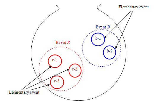
Figure 8-2: Event is a set of elementary-events

 

We explain the reason by the concept of an elementary-event. According to the probability theory, we interpret the event that we take out a ball as an elementary-event. We interpret an event as a set of elementary-events.

 

In order to derive Born rule, we need to find elementary-events of quantum theory. An elementary-event of probability theory generally we cannot divide anymore, so it is expected that an elementary-event of quantum theory also cannot be divided anymore.

 

8.4      Penrose's spin networks

Roger Penrose^[15] proposed spin networks in 1971. According to the spin networks, we express the space as a graph with a line that connects a point and the other point. This graph is called spin network. Since the space-time is discrete, the space-time has a minimum length and minimum time.

 

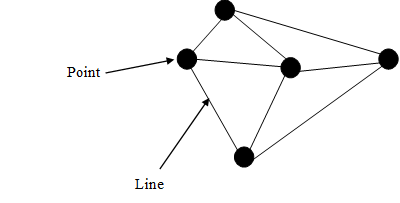
Figure 8-3: Penrose's spin network

 

In this paper, though we do not use a spin network, we assume that space-time is discrete as well as by this theory and the space is a graph that connects the points. In this paper, we assume that the minimum length is Planck length  and the minimum time is Planck time t_P.

 

 

We call the minimum domain that is constructed by the Planck length elementary domain.

 

If the space-time is discrete, we need to review the theory that has been constructed based on the continuous space-time. Therefore, in the next section, we review what happens in the path integral in the case of discrete space-time.

 

8.5      Feynman's path integral

Richard Feynman^[16] proposed path integral in 1948. It provides a new quantization method. In the path integral, we need to take the sum of all the possible paths of the particle.

We express the probability amplitude K (b, a) from the position a to the position b as follows.

 

 

The probability amplitude K (b, a) is called propagator. The symbol Dx (t) represents the sum of the probability amplitudes for all paths. We express the wave functions by the propagator as follows.

 

 

In the path integral, an event that a particle moves from a position a to the other position b is made to correspond to the propagator K (b, a). We get the wave function of time t_b by multiplying the propagator K (b, a) to a wave function of time t_a and integrating it.

 

As shown in the following figure, there is not only a normal path of α but also the other path of β to travel long distance in a short period. Such path might have a speed that is greater than the speed of light. Since the path is contrary to the special relativity, the path is not allowed. In this paper, we call such a movement of the path long distance transition.

 

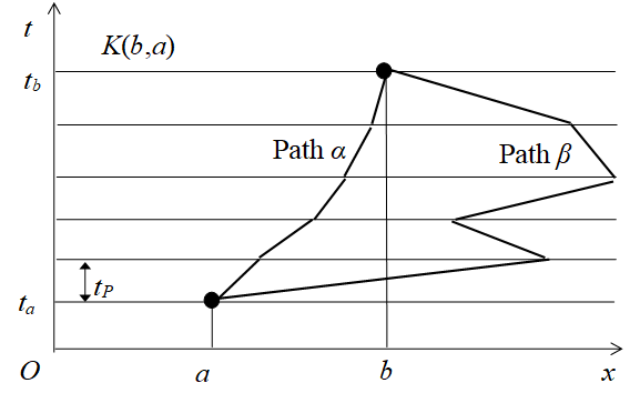
Figure 8-4: Feynman's path integral

 

Generally, the textbook of a path integral explains as follows.

 

The sum of a minutely different path near a path α becomes large. On the other hand, the sum of a minutely different path near a path β becomes small. For this reason, long distance transition is suppressed and the path β does not remain.

 

Then, what happens after the minimum time t_P? We express the propagator from a position a to a position b after a minimum time t_P as follows.

 

 

In this paper, we assume the discrete time. Since we cannot divide minimum time any more, when the departure point and the point of arrival are decided, it cannot take a minutely different path near a path β. For this reason, we cannot suppress long distance transition and the path β remains.

 

Therefore, if we apply the path integral to the discrete space-time and the position of a particle is determined like a delta function of the Dirac, long distance transition occurs after the minimum time t_P.

 

 

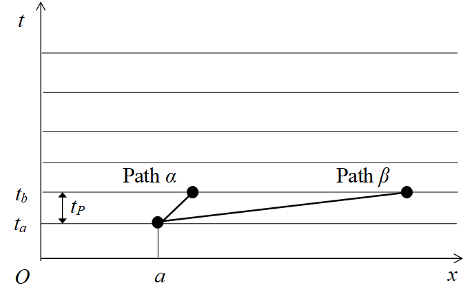
Figure 8-5: Long distance transition in the path integral

 

However, we do not observe the long distance transition. We deduce the reason is that the position of the particle is distributed with a normal distribution like the following figure.

 

Figure 8-6: A wave function of a localized-state

 

Therefore, position x is distributed with deviation Δx, momentum p is also distributed with deviation Δp. According to the Uncertainty Principle, the product of Δx and Δp is close to the Planck constant .

 

 

We call the state of the wave function with a normal distribution localized-state.

 

We express a wave function of a particle with momentum p as follows.

 

We suppose that this particle has a mass m and the velocity v. The momentum is shown below.

We get the following formula by substituting this formula to the wave function.

We express the velocity v by the moving distance x and the Planck length t_P.

We get the following formula by substituting this formula to the wave function.

From the above formula, the wavelength of the wave function is long at the short range. On the other hand, the wavelength of the wave function is short at the long range.

 

In the short distance, the sum of the path integral of localized-state becomes large. On the other hand, in long distance, the sum of the path integral of localized-state becomes small. We call this phenomenon “suppression of long distance transition due to localized-states.”

 

If the state is localized-state, the long distance transition does not occur after the minimum time t_P. Therefore, the localized-state is localized near the place after the time t_P. For this reason, we deduce that network structure of the path integral is realized, as shown in the following figure.

 

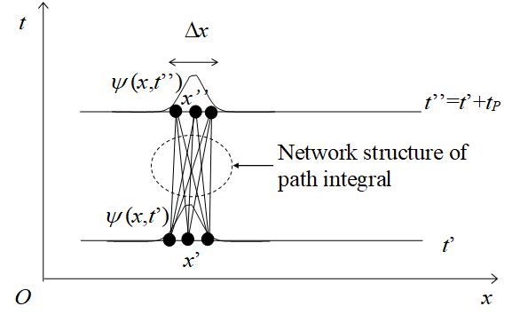
Figure 8-7: Network structure of the path integral

 

In this paper, we call the network structure of “path network structure of the path integral.”

 

We suppose that there is an event AB that is a transition from a state A to a state B. If the state A has three positions and the state B has three positions, the event AB has 3 × 3 = 9 paths.

 

In "network structure of the integral path," the number of paths is the square of the number of positions. On the other hand, according to Born rule, the probability becomes the square of the absolute value of the wave function. In this paper, we discuss the similarities of these squares.

 

8.6      Dirac's quantum field theory

Paul Dirac^[17] proposed the quantum field theory to explain the emission and absorption of electromagnetic waves in 1927. We express the fundamental commutation relation^[18] of the quantum field theory in the case of one-dimensional space as follows.

 

 

Then ψ is the field and π is the conjugate operator of the field ψ. The variable x and y are positions. The function δ is Dirac's delta function.

 

This commutation relation is similar to the following commutation relation between position x and momentum p.

 

 

This indicates that field ψ is a physical quantity that has a property similar to the position x. In this paper, we call the physical quantity “positional physical quantity.”

 

We got a field ψ(x) by the first quantization for the position x. On the other hand, the field ψ(x) is "positional physical quantity" like the position x. Therefore, we get a new field Ψ(x, ψ(x)) by the second quantization for the field ψ. We call the field Ψ(x, ψ(x)) the second wave function. We express the second wave function Ψ(x, ψ(x)) in the following figure.

 

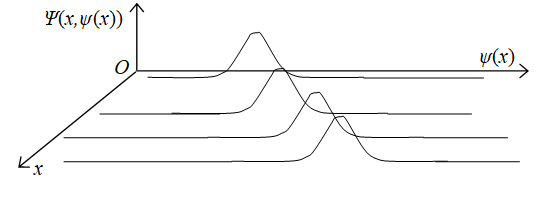
Figure 8-8: The second wave function

 

It is possible to interpret the second wave function Ψ(x, ψ(x)) as a functional Φ [ψ(x)]. We express the functional Φ [ψ(x)] by the many-particle wave function ψ (x₁, x₂, x₃, …, x_n) approximately. To argue a point easily, we use many-particle wave functions by this paper.

 

8.7      Kaluza-Klein theory

Theodor Kaluza^[19] proposed in 1921 and Oskar Klein^[20] proposed in 1926 the extra space like a one-dimensional circle, in order to unify the electromagnetic field and gravity. This theory is called Kaluza-Klein theory.

We express a new space M⁴×S¹ by using a normal four-dimensional space-time M⁴ and an extra space S¹ like a one-dimensional circle as follows.

 

 

Figure 8-9: Kaluza-Klein theory

 

9       Appendix: Review of existing ideas (part 2)

9.1      Euler’s formula

Euler published the following formula in 1748.

(Euler’s formula)

Imaginary number i satisfies the following equation.

We express the complex number as follows.

We express the complex conjugate as follows.

We express the complex function as follows.

We express the square of the absolute value of the complex number as follows.

We use the following symbols as follows.

 

9.2      Cauchy-Riemann equation

Augustin Louis Cauchy[21] introduced the following equation in 1814 for complex analysis. Riemann[22] used the following equation in 1851.

(Cauchy-Riemann equation)

We express the above equation shortly as follows.

(Cauchy-Riemann equation)

 

Cauchy introduced the following formula.

(Cauchy's integral formula)

S is the contour path.

 

9.3      Hamilton’s Quaternion

William Rowan Hamilton[23] proposed the quaternion in 1843.

We express the quaternion as follows.

We express the quaternion conjugate as follows.

We express the quaternion function as follows.

We express the square of the absolute value of the quaternion as follows.

We use the following symbols as follows.

 

9.4      Cauchy-Riemann-Fueter equation

Fueter [24] introduced the following equation in 1934 for quaternionic analysis.

(Cauchy-Riemann-Fueter equation)

We express the above equation shortly as follows.

(Cauchy-Riemann-Fueter equation)

 

Fueter introduced the following formula.

(Cauchy-Fueter integral formula)

Here, S³ is a three-dimensional closed surface. The detail of the quaternionic analysis was described in the Anthony Sudbery’s paper[25] in 1979.

 

We use the following formula.

(Integral formula of quaternion)

Here, u is a unit quaternion.

 

Please refer to the following paper for the integral formula of quaternion.

・Derivation of the reflection integral equation of the zeta function by the quaternionic analysis [2014/5/18]

https://xseek-qm.net/Quaternion_e.htm

 

9.5      Cartan's differential form

Elie Cartan^[26] defined differential form in 1899 in order to describe manifold by the method that is independent to the coordinates.

Though the differential form dω is infinitesimal, we use difference form δω of finitesimal

 

We express the surface area A of the manifold S as follows.

We express the difference form δS of the surface area of the manifold S as follows.

 

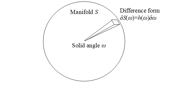
Figure 9-1: Manifold

 

Here, we express the difference form δS₁ of the surface area of the manifold S₁ as follows.

Then, we express the difference form δS₂ of the surface area of the manifold S₂ as follows.

 

We get the following manifold S as the superposition of the manifold S₁ and S₂.

 

We sum the complex numbers of wave functions every position for the superposition of a wave function. Therefore, we deduce that we sum the surface areas of manifolds at every solid angle for the superposition of manifolds.

 

Then, we express the difference form δS of the manifold S as follows.

Therefore, we have the following formula for the spherical harmonics.

We define the superposition of the manifolds by the above formula.

 

10    Appendix: Hierarchical universe

10.1   Universe of Two-dimensional space-time

10.1.1     Closed path of Two-dimensional space-time

We consider the universe U of two-dimensional space-time.

 

We express the world lines of the particle by a complex number.

We express the wave function of this particle as follows.

We suppose that particles are generated by pair production and destroyed by pair annihilation.

 

 

Figure 10-1: Pair production and pair annihilation

 

 

We express the closed path C by the circle C of radius R as follows.

 

Figure 10-2: Closed path C

 

We express this closed path as follows.

We express the circumference a of this circle C as follows.

Here we introduce the complex solid angle ω.

We express the closed path as follows.

Then we express the circumference a of this circle C as follows.

We express the difference form of the circumference a as follows.

 

10.1.2     Introduction of the absolute value of wave function

We introduce a circle S as an extra space like Kaluza-Klein theory.

 

We express the point on the circle C by matrix representation of a complex number as follows.

We call the circle an amplitude circle or an amplitude 1-sphere.

 

Figure 10-3: Amplitude 1-sphere S

 

We express the circumference A of the amplitude 1-sphere S by the radius R and the solid angle Ω as follows.

If the radius R is the function of r and ω, the circumference A becomes the function of r and ω.

We express the difference form δS of the sphere S.

We interpret the circumference A as the absolute value of the wave function.

 

10.1.3     Introduction of the phase of wave function

In order to introduce the phase of wave function, we rotate the sphere S. by the rotational transform angle Φ. We transform the sphere S to the new sphere S’ by the rotational transform which depends on ω.

We define the rotational transform of the rotational transform angle Φ that depends on ω as follows.

We express the function Φ (ω) by the natural number n as follows.

We interpret the rotational angle Φ as the phase of the wave function.

 

We transform the sphere S by the rotational transform as follows.

 

Figure 10-4: Rotation of the amplitude 1-sphere S

 

 

We define the superposition of a sphere S₁ and a sphere S₂ as follows.

The superposition of the sphere and the sphere that is rotated by the angle 180 degrees is zero.

 

The direct product of the closed path C of the particle and the sphere S becomes a torus T.

We call this torus T a torus world-sheet.

 

 

Figure 10-5: The torus world-sheet

 

 

Here, we introduce the following new solid angle ν.

Here we introduce the following new solid radius ρ.

Here we introduce the following new function f (ρ, ν).

We express the torus world-sheet T by the function f (ρ, ν) as follows.

The torus world-sheet is twisted like a helical torus as the following figure.

 

Figure 10-6: The torus world-sheet is twisted like a helical torus.

 

This dimension of the torus world-sheet is same as the dimension of the universe because the universe is two-dimensional space-time in this section.

 

Here we use a surprising idea.

 

We interpret the torus world-sheet as a new space-time. We call the space-time toric space-time.

We interpret the toric space-time an independent universe. We call the universe the second universe.

 

It is possible to construct the third and the forth universe in the same way that we construct the second universe. We construct many universes by repeating the same way. We call these universes hierarchical universe.

 

10.1.4     Hierarchical universe

We show the hierarchical universe as follows.

Figure 10-7: Hierarchical universe

 

We express the above hierarchical universe by the following symbol.

 

 

10.1.5     Equations

We express the position s by the complex number as follows.

Then the wave function becomes a complex function.

We assume that the complex function is an analytic function.

Analytic functions satisfy the Cauchy-Riemann equation.

(Cauchy-Riemann equation)

We call the equation path differential equation.

 

We define the complex conjugate as follows.

Then we express the path differential equation shortly as follows.

 

Analytic function satisfy the Cauchy's integral formula.

(Cauchy's integral formula)

S is the contour path.

We interpret the Cauchy's integral formula as the path integral equation of Feynman’s path integral.

 

 

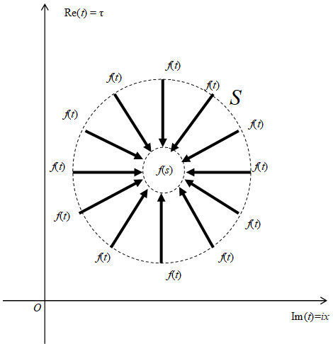
Figure 10-8: The path integral equation of Feynman’s path integral

 

We interpret that the particle on the circle S transit from the position t to the position s for the long distance directly.

We call the new interpretation the path integral of space-time view that is different from the traditional Feynman’s path integral.

 

It is possible to use these equations for wave functions of each universe because the wave functions of each universe are complex functions.

 

 

10.2   Universe of four-dimensional space-time

10.2.1     Closed path of four-dimensional space-time

We consider the universe U of four-dimensional space-time.

 

We express the world lines of the particle by quaternion.

We express the wave function of this particle as follows.

We suppose that particles are generated by pair production and destroyed by pair annihilation.

 

 

Figure 10-9: Pair production and pair annihilation

 

 

We express the closed path s by the circle C of radius r as follows.

 

Figure 10-10: Closed path C

 

We express this closed path as follows.

We express the circumference a of this circle C as follows.

Here we introduce the quaternionic solid angle ω.

We express the closed path as follows.

Then we express the circumference a of this circle C as follows.

We express the difference form of the circumference a as follows.

 

10.2.2     Introduction of the absolute value of wave function

We introduce a three-dimensional sphere (3-sphere) S as an extra space like Kaluza-Klein theory.

 

We express the point S on the 3-sphere by matrix representation of quaternion.

 

 

We call the circle amplitude 3-sphere.

 

Figure 10-11: Amplitude 3-sphere S

 

We express the circumference A of the amplitude 3-sphere S by the radius R and the solid angle Ω as follows.

If the radius R is the function of r and ω, the circumference A becomes the function of r and ω.

We express the difference form δS of the sphere S.

We interpret the circumference A as the absolute value of the wave function.

 

10.2.3     Introduction of the phase of wave function

In order to introduce the phase of wave function, we rotate the sphere S. by the rotational transform angle Φ. We transform the sphere S to the new sphere S’ by the rotational transform which depends on ω.

 

We define the rotational transform of the rotational transform angle Φ that depends on ω as follows.

We express the function Φ (ω) by the natural number n as follows.

We interpret the rotational angle Φ as the phase of the wave function.

 

We transform the sphere S by the rotational transform as follows.

 

Figure 10-12: Rotation of the amplitude 3-sphere S

 

 

We define the superposition of a sphere S₁ and a sphere S₂ as follows.

The superposition of the sphere and the sphere that is rotated by the angle 180 degrees is zero.

 

The direct product of the closed path C of the particle and the sphere S becomes a manifold like a torus T.

We call this manifold T a torus world-sheet.

 

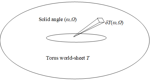
Figure 10-13: The torus world-sheet

 

Here we introduce the following new solid angle ν.

Here we introduce the following new solid radius ρ.

Here we introduce the following new function f (ρ, ν).

We express the torus T by the function f (ρ, ν) as follows.

The torus world-sheet is twisted like a helical torus as the following figure.

 

Figure 10-14: The torus world-sheet is twisted like a helical torus.

 

This dimension of the torus world-sheet is same as the dimension of the universe because the universe is four-dimensional space-time in this section.

 

Here we use a surprising idea.

 

We interpret the torus world-sheet as a new space-time. We call the space-time toric space-time.

We interpret the toric space-time an independent universe. We call the universe the second universe.

 

It is possible to construct the third and the forth universe in the same way that we construct the second universe. We construct many universes by repeating the same way. We call these universes hierarchical universe.

 

10.2.4     Hierarchical universe

We show the hierarchical universe as follows.

 

Figure 10-15: Hierarchical universe

 

We express the above hierarchical universe by the following symbol.

 

 

10.2.5     Equations

We express the position s by the quaternion number as follows.

Then, the wave function becomes a quaternionic function.

We assume that quaternionic functions are analytic functions.

Analytic functions satisfy the Cauchy-Riemann-Fueter equation.

(Cauchy-Riemann-Fueter equation)

We call the above equation path differential equation in this paper.

 

We define the quaternionic conjugate as follows.

Then we express the path differential equation shortly as follows.

Analytic functions satisfy the integral formula of quaternion.

(Integral formula of quaternion)

 

Here, u is a unit quaternion.

We interpret the integral formula of quaternion as the path integral equation of Feynman’s path integral.

 

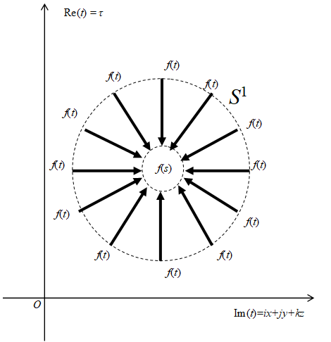
Figure 10-16: Path integral equation of Feynman’s path integral

 

We interpret that the particle on the circle S¹ transit from the position t to the position s for the long distance directly.

We call the new interpretation a space-time view path integral that is different from the traditional Feynman’s path integral.

 

It is possible to use these equations for the wave function of each universe because the wave functions of each universe are quaternionic functions.

 

 

10.3   Normal space

We express the surface area a of the normal space U as follows.

We express the difference form of the normal space U as follows.

Here we replace the r³ to the function f (ω).

Then we express the following formula.

We interpret the above formula like the following figure.

We call the interpretation manifold view.

 

Figure 10-17: Manifold view of the normal space U

 

Here we rewrite the formula as follows by a new function f (r, ω).

We interpret the above formula like the following figure.

We call the interpretation spherical harmonics view.

 

Figure 10-18: Spherical harmonics view of the normal space U

 

In the spherical harmonics view, we interpret the function f (r, ω) as the spherical harmonics.

The spherical harmonics f (r, ω) is the solution of the Laplace equation of the spheric polar coordinates.

Therefore, spherical harmonics f (r, ω) satisfies the following Laplace equation.

Here, we used the following symbols.

 

 

 

10.4   Wave space-time

We express the normal space-time U by the radius r and the solid angle ω as follows.

We express the amplitude 3-sphere S by the radius R and the solid angle Ω as follows.

We define the wave space-time W as the direct product of the normal space-time U and the amplitude 3-sphere S as follows.

Here we introduce the new solid angle.

Here we introduce the new radius.

Here we introduce the new function.

Then we express the wave space-time shortly.

 

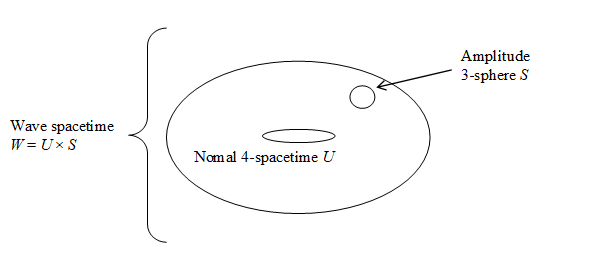
Figure 10-19: Wave space-time

 

The spherical harmonics g (ρ, ν) is the solution of Laplace equation of the spheric polar coordinates.

Therefore, the spherical harmonics g (ρ, ν) satisfies the following harmonic equation.

Here, we used the following symbols.

 

11    Appendix: Terms

11.1   Definition of Terms

We define terms in the following table.

 

Table 11-1: Normal space and wave space

 

Table 11-2: Elementary-state and so on

 

We abbreviate an elementary-state particle to a state-element.

We abbreviate an elementary-world particle to a world-element.

 

11.2   Arrangement of Terms

We arrange terms in the following table.

 

Table 11-3: Elementary-state and so on

 

12    Acknowledgment

In writing this paper, I thank from my heart to TY and NS who gave valuable advice to me.

 

 

 

 

 

13    References