Why does the square of the imaginary unit i become -1?

 

Home  >  Quantum mechanics  >  Do imaginary numbers exist?

 

2019/3/2

Published 2014/6/29

Koji Sugiyama

 

I explain why the square of the imaginary unit i becomes -1.

 

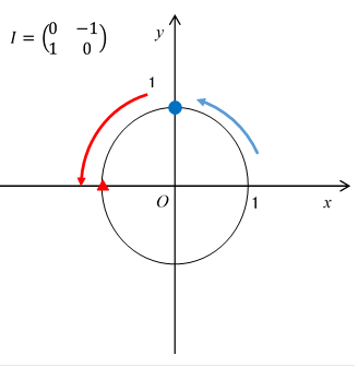
Figure 2-9: A rotation matrix rotates 90 degrees counter-clockwise.

 

Euler introduced symbol i of the imaginary unit in 1777 and showed the following formula.

i² = -1

 

This is a very mysterious formula. Why does the square of the number becomes minus one?

Euler, Gauss, and Hamilton have solved the secret of this formula. I would like the people to read this article, who want to know the secret of the formula.

 

The points are as follows.

(1) We interpret the imaginary unit as an abbreviation of a matrix.

(2) We interpret the imaginary unit as the 90 degrees turn of a picture.

(3) We interpret minus one as the 180 degrees turn of a picture.

(4) When we rotate the picture 90 degrees twice, it becomes a turn 180 degrees.

 

To understand the reason that an imaginary number is interpreted as an abbreviation of a matrix, I would like to explain the geometrical interpretation of a matrix in this article.

 

Contents

1.     Introduction. 1

2.     Matrix. 1

2.1.      Matrix as the abbreviation of linear transformation. 1

2.2.      Operation rule of a matrix. 1

2.3.      Circle transformation diagram of a matrix. 1

2.4.      Rotation. 1

2.5.      Expansion. 1

2.6.      Expanding unit matrix. 1

2.7.      Rotational unit matrix. 1

3.     Complex numbers. 1

3.1.      Complex numbers as an abbreviation of the matrices. 1

3.2.      Euler's formula. 1

4.     Conclusion. 1

5.     Supplement 1

5.1.      Matrix. 1

5.1.1.       What is the transposed matrix?. 1

5.1.2.       What is the symmetric matrix?. 1

5.1.3.       What is the determinant?. 1

5.1.4.       What are the eigenvectors and the eigenvalues?. 1

5.1.5.       What is the characteristic equation?. 1

5.1.6.       What is the singular value decomposition?. 1

5.2.      Complex numbers. 1

5.2.1.       What is real numbers?. 1

5.2.2.       What are imaginary numbers?. 1

5.2.3.       What are complex numbers?. 1

5.3.      Complex matrices. 1

5.3.1.       What is the complex conjugate?. 1

5.3.2.       What is the adjugate matrix?. 1

5.3.3.       What is the self-adjoint matrix?. 1

6.     Appendix. 1

6.1.      Quaternions. 1

6.1.1.       What are the quaternions?. 1

6.1.2.       What is the quaternion conjugate?. 1

6.1.3.       What is the inner product?. 1

6.1.4.       What is the cross product?. 1

6.2.      Complex numbers. 1

6.2.1.       Geometrical interpretation of complex numbers. 1

6.2.2.       The inner product of complex numbers. 1

6.2.3.       The cross product of complex numbers. 1

7.     Acknowledgment 1

8.     Reference document 1

 

 

In this article, I will explain the following formula is satisfied.

(Equation of the imaginary unit)

 

To understand a matrix, I would like to consider transformation of a picture.

 

We move a point (x, y) to a point (x', y') as follows.

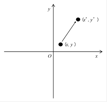
Figure 2-1: A matrix moves a point (x, y) to a point (x', y').

 

We express this transformation in the following expression.

This transformation is called a linear transformation.

 

The expression of a linear transformation is complicated. Then, in order to write more simply, we express it by the following abbreviation.

We call the abbreviation of the linear transformation as the above expression the matrix.

 

This matrix moves a point (1, 0) and a point (0, 1) as follows.

 

A movement destination of a point (1, 0) becomes the coordinate (a, c) which is made from a, c in the first column of the matrix.

A movement destination of a point (0, 1) becomes the coordinate (b, d) which is made from b, d in the second column of the matrix.

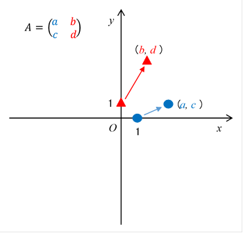
Figure 2-2: A movement destination of a point (1, 0) becomes the component (a, c) of the matrix and a movement destination of a point (0, 1) becomes the component (b, d) of the matrix.

 

I would like to derive the operation rule of a matrix from the linear transformation.

 

A linear transformation is as follows.

We will transform the above point (x', y') once again.

Next, we substitute the formula (2.5) into the formula (2.6). Then, we obtain the following formula.

 

The formula (2.5), (2.6), and (2.7) are complicated. Then, in order to write more simply, we express it by the following abbreviation.

 

On the other hand, we interpret the left side of an equation (2.8) as one value, and substitute the value into the formula (2.9). Then, we obtain the following formula.

We compare the formula (2.10) and the formula (2.11). Then, we obtain the following formula.

We define the operation rule of the matrix by the above equation.

 

British mathematician Arthur Cayley defined this operation rule of the matrix in 1588. [1]

 

It is difficult to indicate a matrix because the matrix transforms the whole picture.

Then, we observe the unit circle that is transformed by the matrix.

 

For example, we consider the following matrix.

 

How does this matrix transform the following unit circle?

It is the following ellipse.

 

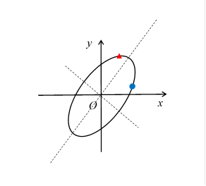
Figure 2-3: Circle transformation diagram of a matrix

 

 

The blue circle mark ● means the movement destination of a point (1, 0). The red triangle mark ▲ means the movement destination of a point (0, 1). The dotted lines are major axis and minor axis of the ellipse. In this article, we call the expression like this "circle transformation diagram."

 

When we see the above figure, the major axis of the ellipse seems to be an eigenvector. However, it is not always so. Generally, the major axis is different from an eigenvector like the following figure.

 

 

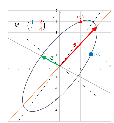
Figure 2-4: The major axis of ellipse is different from an eigenvector of a matrix

 

We are able to express a general matrix by the following four kinds of operation, according to the singular value decomposition to be described.

 

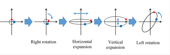
Figure 2-5: We are able to decompose a matrix to right rotation, horizontal expansion, vertical expansion, and left rotation.

 

We are able to express a matrix by rotation and expansion. Therefore, I explain the rotation and the expansion in the following sections.

 

We consider the following matrix.

This is called rotational matrix. We express the rotational matrix by the following matrix.

The circle transformation diagram is shown below.

 

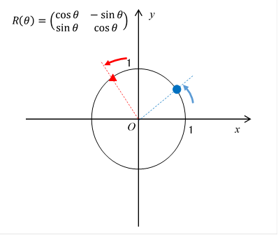
Figure 2-6: Rotational matrix

 

We express the right rotation as follows.

 

We express the matrix that expands the x-axis direction into two times.

In this article, we call this matrix horizontal expanding matrix.

 

 

The circle transformation diagram is shown below.

 

Figure 2-7: Horizontal expanding matrix expands the picture horizontally.

 

We are able to make a matrix that expands the picture vertically by the same method of the horizontal expanding matrix. In this article, we call this matrix the vertical expanding matrix.

 

We consider the following matrix.

We express the matrix by the real number time of the unit matrix.

In this article, we call this matrix the expanding matrix.

In this article, we call the unit matrix the real number unit matrix or the expanding unit matrix.

 

If the vertical and horizontal expansion rate of a transformation is same, we express the transformation by the following matrix.

The circle transformation diagram is shown below.

 

 

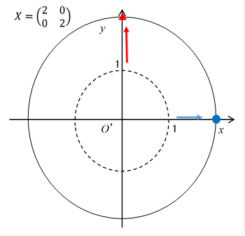
Figure 2-8: An expanding matrix expands equally.

 

 

We consider the following matrix.

In this article, we call the unit matrix the imaginary number unit matrix or the rotational unit matrix.

 

We express the turn of 90 degrees by the following matrix.

The circle transformation diagram is shown below.

 

Figure 2-9: A rotation matrix rotates 90 degrees counter-clockwise.

 

We are able to decompose any matrix to the following transformations.

(1) Right rotation

(2) Horizontal expansion

(3) Vertical expansion

(4) Left rotation

 

This decomposition is called the singular value decomposition (SVD).

 

If the horizontal expansion rate is equal the vertical expansion rate, we are able to commute rotation to expansion. In the case, we are able to decompose any matrix to the following transformations.

(1)   Rotation

(2)   Expansion

 

This commutative property is the origin of the commutative property of complex numbers those will be described in the following section.

 

In order to understand the reason to interpret complex numbers as an abbreviation of matrices, we consider the following matrix.

In this article, we call this matrix the imaginary unit matrix, or rotation unit matrix.

 

This matrix satisfies the following equation.

In this article, we call the matrix E the expanding unit matrix.

 

Here we define the following matrix.

In this article, we call this matrix Z the expanding rotation matrix. We use the following abbreviation for the matrix.

We called "the abbreviation of expanding rotation matrix" the complex number.

The original matrix is called "matrix representation of complex numbers."

 

Leonhard Euler [2] has discovered the following formula in 1748.

(Euler's formula)

Matrix representation of complex numbers is as follows.

We are able to express the right-hand side by the components as follows.

Right-hand side is equal to the following rotation matrix.

 

In this article, we explain the following contents.

 

- We are able to interpret the complex numbers as the abbreviation of expanding rotation matrices.

 

Therefore, we are able to interpret the imaginary unit as the abbreviation for the imaginary unit matrix. We are able to interpret the imaginary unit as 90-degree rotation of the image. We are able to interpret the -1 as 180-degree rotation of the image, too.

 

The double 90-degree rotation is equal to 180-degree rotation. Therefore, we understand the reason why the square of the imaginary unit becomes -1 geometrically.

 

 

The transposed matrix is the matrix obtained by exchange components of the rows to columns of a matrix.

We may also express the transposed matrix as follows.

However, this article will adopt the following notation.

 

What is the difference between the transposed matrix and the original matrix? We introduce the following matrix in order to consider it.

We interpret the transposed matrix as follows.

 

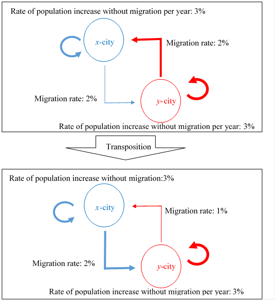
Figure 5-1: The transposed matrix

 

 

In the above figure, the migration rate from x-city to y-city is not equal to the migration rate from y-city to x-city. This -operation to replace these migration rates is a transposition.

 

If these migration rates are same, the matrix becomes the symmetric matrix that will be described below.

 

If the transposed matrix is equal to the original matrix, the matrix is called the symmetric matrix.

The following matrix is the symmetric matrix.

In the case of the symmetric matrix, the major axis of the circle transformation diagram is equal to the eigenvector.

 

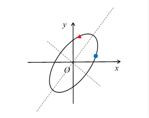
Figure 5-2: In the case of the symmetric matrix, the major axis of the circle transformation diagram is equal to the eigenvector.

 

Augustin-Louis Cauchy [3] has proven that all eigenvalues of the symmetric matrix are real numbers in 1829.

 

 

We are able to interpret a determinant as the extension rate of an area by a matrix.

 

We express the determinant as follows.

Matrix equation Augustin-Louis Cauchy [4] has defined in 1815.

 

We are able to interpret a determinant of a two-dimensional matrix as an area expansion rate.

We are able to interpret a determinant of 3-dimensional matrix as a volume expansion rate.

 

Eigenvectors are vectors whose direction does not change by transformation of a matrix. Eigenvalues are expansion rates of the eigenvectors.

 

In the case of the symmetric matrix, the major axis of the circle transformation diagram is equal to the eigenvector.

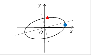
Figure 5-3: In the case of the symmetric matrix, the major axis of the circle transformation diagram is equal to the eigenvector.

 

A characteristic equation is an equation we use in order to obtain the eigenvalues of a matrix. The characteristic equation is shown below.

We express the characteristic equation by the components as follows.

Why are we able to derive the eigenvalues by the characteristic equation? In order to understand this reason, we observe the change of the matrix A−λE by changing the variable λ.

 

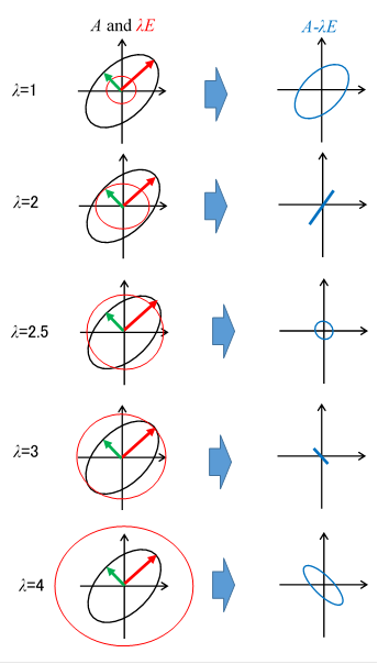
Figure 5-4: A mechanism that we are able to derive the eigenvalues by the characteristic equation.

 

The black ellipse is the circle that is transformed by the matrix A. The red circle is the circle that is transformed by the matrix λ E. The blue ellipse is the circle that is transformed by the matrix A−λE. The red arrows and the green arrows are eigenvectors with the length of the eigenvalues. When the radius of the red circle is equal to the length of one of these arrows, the determinant is equal to zero.

 

If the area of the blue circle is zero, the area extension rate is zero. Therefore, we are able to interpret that we search the value of the variable λ that the area extension rate is zero by changing the variable λ.

 

In the case of the symmetric matrix, an eigenvector is equal to the major axis of the ellipse. Therefore, the radius of the red circle is equal to the length of one of these arrows when the red circle is in contact with the black ellipse.

 

A singular value decomposition is the following decomposition.

 

- We are able to decompose any matrix M to rotation matrix R (-θ), the diagonal matrix D, and the rotation matrix .

 

We are able to express a general matrix by the following four kinds of operation by the singular value decomposition.

 

Figure 5-5: We are able to decompose a matrix to right rotation, horizontal expansion, vertical expansion, and left rotation.

 

The horizontal expansion rate and vertical expansion rate are called the singular values. They are generally not equal to the eigenvalues. In the case of the symmetric matrix, horizontal expansion rate and vertical expansion rate are eigenvalues.

 

Eugenio Beltrami [5] and Camille Jordan [6] have discovered the singular value decomposition independently in 1873 and 1874.

 

The real number is an abbreviation of "real number times of the expanding unit matrix."

The expanding unit matrix is as follows.

We use the following abbreviation 1 to express this matrix.

We express the matrix of the real numbers as follows.

We use the following abbreviation to express this matrix of the real numbers.

 

 

The imaginary number is an abbreviation of "real number times of the rotation unit matrix."

Rotation matrix is as follows.

We use the following abbreviation i to express this matrix.

We express the matrix of the imaginary numbers as follows.

We use the following abbreviation to express this matrix of the imaginary numbers.

 

 

The complex number is an abbreviation of "the expansion rotational matrix."

The expanding unit matrix is as follows.

The expansion rotational matrix is as follows.

We express the matrix of the complex numbers as follows.

We use the following abbreviation to express this matrix of the complex numbers.

 

 

The complex conjugate consists of changing the sign of the imaginary part of the complex number.

 

Now, we express a complex number as follows.

In mathematics, the complex conjugate is described as follows.

On the other hand, in physics the complex conjugate is described as follows.

This article adopts the following notation of mathematics.

 

In the case of the matrix representation of complex numbers, complex conjugate is expressed by the following transposed matrix.

 

We are able to interpret the complex conjugate as the transposed matrix. Therefore, we need to change any complex number to the complex conjugate when we transpose any matrix.

 

The adjugate matrix is the transposed matrix obtained by taking the complex conjugate of each entry.

This matrix is also known as the following names.

 

- Hermitian conjugate

- Hermitian transpose

- Hermitian adjoint

- Conjugate transpose

 

Now, we express a matrix as follows.

In mathematics, the adjugate matrix is described as follows.

 

In physics, the adjugate matrix is described as follows.

This article adopts the following notation of mathematics.

 

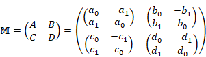
We define the following matrix  with the entries of matrix representations of complex number A, B, C, and D.

 

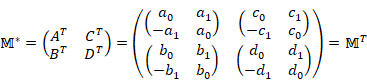
In the case of the matrix with the entries of matrix representations of complex numbers, adjugate matrix is the transposed matrix.

 

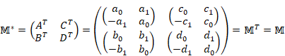
If an adjugate matrix is equal to the original matrix, the matrix is called self-adjoint matrix.

This matrix is also known as Hermitian matrix.

 

Charles Hermite [7] showed that all the eigenvalues of the Hermitian matrix are real numbers in 1855.

 

We define the following matrix  with the entries of matrix representations of complex number A, B, C, and D.

 

In the case of the matrix with the entries of matrix representations of complex numbers, Hermitian matrix is the symmetric matrix.

 

Hamilton introduced quaternion in 1843. We are able to interpret a quaternion as an abbreviation of the following matrix.

We express the matrix of a quaternion as follows.

We use the following abbreviation to express a quaternion.

 

The quaternion conjugate consists of changing the sign of the imaginary part of the quaternion.

Physically, it means space reflection.

 

In the case of the matrix representation of the quaternions, quaternion conjugate is an adjugate matrix.

 

The inner product of three-dimensional vector u and the three-dimensional vector v is defined as follows.

However, why the inner product definition as described above?

 

In order to understand this reason, I would like to consider the following the division of quaternion q by quaternion p.

We define the following rotation by the quaternion R.

We rotate the quaternion p to p'.

We rotate the quaternion q to q'.

The quaternion s is invariant for the rotation R.

We modify the quaternion s as follows.

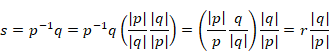
On the other hand, we are able to express the quaternion s as follows.

The rotation R does not change the absolute values of the quaternions p and q. Therefore, the quaternion r is invariant for the rotation R.

 

We make the following equation by the formula (6.20) and (6.21).

We modify the above equation as follows.

The absolute values of the quaternions p and q are invariant for the rotation R.

The quaternion r is invariant for the rotation R, too.

Therefore, the left-hand side is invariant for the rotation R.

 

In this article, we call the left-hand side as rotation invariant product. We are able to confirm that the rotation invariant product is invariant for rotation as follows.

The real part and imaginary part of the rotation invariant product is invariant for the rotation.

 

We are able to interpret the inner product of three-dimensional vectors as the real part of the quaternion of pure imaginary.

 

The cross product of three-dimensional vector u and the three-dimensional vector v is defined as follows.

However, why cross product definition as described above?

 

In fact, we are able to interpret the cross product of three-dimensional vector as a sign inversion of the imaginary part of the rotation invariant product of the quaternion of pure imaginary.

 

 

 

Norwegian surveyor Caspar Wessel published the complex plane in 1797. The complex plane is the plane to express complex numbers geometrically.

 

Figure 6-1: The complex number a+bi exists as a point (a, b) in the complex plane.

 

French mathematician Jean-Robert Argand also published the complex plane in 1806. German mathematician Carl Friedrich Gauss used the complex plane in 1831.

 

Hamilton express the complex number a + bi as (a, b), and define the operation of the addition and the product as follows.

 

 

The inner product of three-dimensional vector u and the two-dimensional vector v is defined as follows.

However, why the inner product definition as described above?

 

In order to understand this reason, I would like to consider the following the division of complex number q by complex number p.

We define the following rotation by the complex number R.

We rotate the complex number p to p'.

We rotate the complex number q to q'.

The complex number s is invariant for the rotation R.

We modify the complex number s as follows.

On the other hand, we are able to express the complex number s as follows.

The rotation R does not change the absolute values of the complex numbers p and q. Therefore, the complex number r is invariant for the rotation R.

 

We make the following equation by the formula (6.20) and (6.21).

We modify the above equation as follows.

The absolute values of the complex numbers p and q are invariant for the rotation R.

The complex number r is invariant for the rotation R, too.

Therefore, the left-hand side is invariant for the rotation R.

 

In this article, we call the left-hand side as rotation invariant product. We are able to confirm that the rotation invariant product is invariant for rotation as follows.

The real part and imaginary part of the rotation invariant product is invariant for the rotation.

 

We are able to interpret the inner product of three-dimensional vectors as the real part of the complex number of pure imaginary.

 

The cross product of three-dimensional vector u and the two-dimensional vector v is defined as follows.

However, why cross product definition as described above?

 

In fact, we are able to interpret the cross product of three-dimensional vector as a sign inversion of the imaginary part of the rotation invariant product of the complex number of pure imaginary.

 

 

 

In writing this paper, I thank from my heart to NS who gave valuable advice to me.

 

[1]	Cayley, Arthur, "A Memoir on the Theory of Matrices," A Philosophical Transactions of the Royal Society of London, vol. 148, pp. 17-37, 1858.
[2]	Euler, Leonhard, "Introduction to the Analysis of the Infinite (Introductio in analysin infinitorum)," Opera Omnia, vol. 1, no. 8, pp. 92-105, 1748.
[3]	Cauchy, Augustin-Louis, "On the equation which helps one determine the secular inequalities in the movements of the planets (Sur l'equation a l'aide de laquelle on determine les inegalites seculaires)," Oeuvres Completes, vol. 2, no. 9, pp. 174-195, 1829.
[4]	Cauchy, Augustin-Louis, "Memoire sur les fonctions qui ne peuvent obtenir que deux valeurs egales et des signes contraires par suite des transpositions operees entre les variables qu'elles renferment," J Ecole Polytech, vol. 10, pp. 29-112, 1815.
[5]	Beltrami, Eugenio, "Sulle funzioni bilineari," Giornale di Matematiche ad Uso degli Studenti Delle Universita, vol. 11, pp. 98-106, 1873.
[6]	Jordan, Camille, "Memoire sur les formes bilineaires," Journal de Matheantiques Purse, Deuxieme Serei, vol. 19, pp. 35-54, 1874.
[7]	Hermite, Charles, "Remarque sur un theoreme de M. Cauchy," C.R. Acad. Sci. Paris, vol. 41, pp. 181-183, 1855.
[8]	Descartes, René, "La Géométrie," Discours de la méthode, pp. 376-493, 1637.
[9]	Sylvester, James Joseph, "On The relation between the minor determinants of linearly equivalent quadratic functions," Philos. Magazine, vol. I, no. 4, pp. 295-305, 1851.